Picket Fence#

Overview#

The picket fence module is meant for analyzing EPID images where a “picket fence” MLC pattern has been made. Physicists regularly check MLC positioning through this test. This test can be done using film and one can “eyeball” it, but this is the 21st century and we have numerous ways of quantifying such data. This module attains to be one of them. It can load in an EPID dicom image (or superimpose multiple images) and determine the MLC peaks, error of each MLC pair to the picket, and give a few visual indicators for passing/warning/failing.

Features:

Analyze any MLC type - Both default MLCs and custom MLCs can be used.
Easy-to-read pass/warn/fail overlay - Analysis gives you easy-to-read tools for determining the status of an MLC pair.
Any Source-to-Image distance - Whatever your clinic uses as the SID for picket fence, pylinac can account for it.
Account for panel translation - Have an off-CAX setup? No problem. Translate your EPID and pylinac knows.
Account for panel sag - If your EPID sags at certain angles, just tell pylinac and the results will be shifted.

Concepts#

Although most terminology will be familiar to a clinical physicist, it is still helpful to be clear about what means what. A “picket” is the line formed by several MLC pairs all at the same position. There is usually some ideal gap between the MLCs, such as 0.5, 1, or 2 mm. An “MLC position” is, for pylinac’s purposes, the center of the FWHM of the peak formed by one MLC pair at one picket. Thus, one picket fence image may have anywhere between a few to a dozen pickets, formed by as few as 10 MLC pairs up to all 60 pairs.

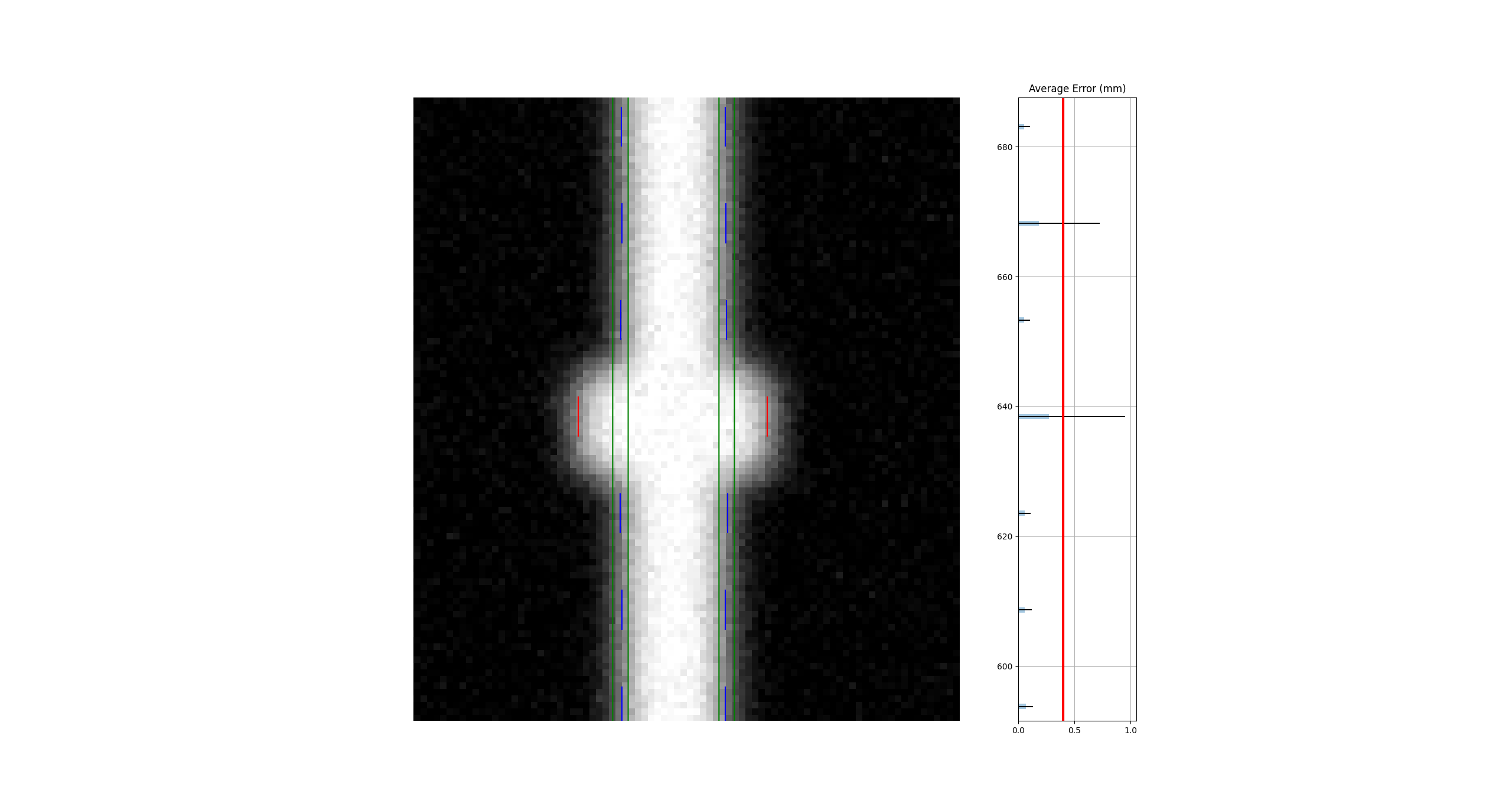
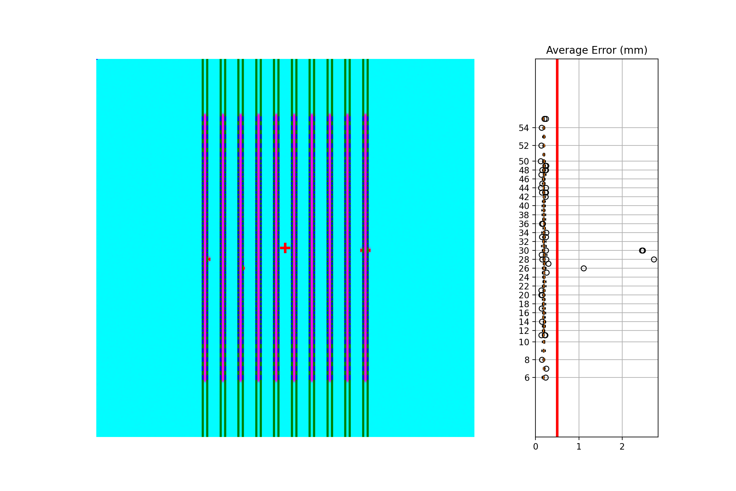
Pylinac presents the analyzed image in such a way that allows for quick assessment; additionally, all elements atop the image can optionally be turned off. Pylinac by default will plot the image, the determined MLC positions, “guard rails”, and a semi-transparent overlay of the MLC error magnitude and translucent boxes over failed leaves. The guard rails are two lines parallel to the fitted picket or side of the picket, offset by the tolerance passed to analyze(). Thus, if a tolerance of 0.5 mm is passed, each guard rail is 0.5 mm to the left and right of the invisible picket. Ideally, MLC positions will all be within these guard rails, i.e. within tolerance, and will be colored blue. If they are outside the tolerance they are turned red with a larger box overlaid for easy identification. If an “action tolerance” is also passed to analyze(), MLC positions that are below tolerance but above the action tolerance are turned magenta.

Additionally, pylinac provides a semi-transparent colored overlay so that an “all clear” or a “pair(s) failed” status is easily seen and not inadvertently overlooked. If any MLC position is outside the action tolerance or the absolute tolerance, the MLC pair/leaf area is colored the corresponding color. In this way, not every position needs be looked at.

Running the Demo#

To run the picketfence demo, create a script or start in interpreter and input:

from pylinac import PicketFence

PicketFence.run_demo()

Results will be printed to the console and a figure showing the analyzed picket fence image will pop up:

Picket Fence Results:
100.0% Passed
Median Error: 0.062mm
Max Error: 0.208mm on Picket: 3, Leaf: 22

(Source code, png, hires.png, pdf)

Finally, you can save the results to a PDF report:

pf = PicketFence.from_demo()
pf.analyze()
pf.publish_pdf(filename="PF Oct-2018.pdf")

Acquiring the Image#

The easiest way to acquire a picket fence image is using the EPID. In fact, pylinac will only analyze images acquired via an EPID, as the DICOM image it produces carries important information about the SID, pixel/mm conversion, etc. Depending on the EPID type and physicist, either the entire array of MLCs can be imaged at once, or only the middle leaves are acquired. Changing the SID can also change how many leaves are imaged. For analysis by pylinac, the SID does not matter, nor EPID type, nor panel translation.

Typical Use#

Picket Fence tests are recommended to be done weekly. With automatic software analysis, this can be a trivial task. Once the test is delivered to the EPID, retrieve the DICOM image and save it to a known location. Then import the class:

from pylinac import PicketFence

The minimum needed to get going is to:

Load the image – As with most other pylinac modules, loading images can be done by passing the image string directly, or by using a UI dialog box to retrieve the image manually. The code might look like either of the following:
```
pf_img = r"C:/QA Folder/June/PF_6_21.dcm"
pf = PicketFence(pf_img)
```
You may also load multiple images that become superimposed (e.g. an MLC & Jaw irradiation):
```
img1 = r"path/to/image1.dcm"
img2 = r"path/to/image2.dcm"
pf = PicketFence.from_multiple_images([img1, img2])
```
As well, you can use the demo image provided:
```
pf = PicketFence.from_demo_image()
```
You can also change the MLC type:
```
pf = PicketFence(pf_img, mlc="HD")
```
In this case, we’ve set the MLCs to be HD Millennium. For more options and to customize the MLC configuration, see Customizing MLCs.
Analyze the image – Once the image is loaded, tell PicketFence to start analyzing the image. See the Algorithm section for details on how this is done. While defaults exist, you may pass in a tolerance as well as an “action” tolerance (meaning that while passing, action should be required above this tolerance):
```
pf.analyze(
    tolerance=0.15, action_tolerance=0.03
)  # tight tolerance to demo fail & warning overlay
```
View the results – The PicketFence class can print out the summary of results to the console as well as draw a matplotlib image to show the image, MLC peaks, guard rails, and a color overlay for quick assessment:
```
# print results to the console
print(pf.results())
# view analyzed image
pf.plot_analyzed_image()
```
which results in:

(Source code, png, hires.png, pdf)

The plot is also able to be saved to PNG:
```
pf.save_analyzed_image("mypf.png")
```
Or you may save to PDF:
```
pf.publish_pdf("mypf.pdf")
```

Analyzing individual leaves#

Historically, MLC pairs were evaluated together; i.e. the center of the picket was determined and compared to the idealized picket. In v3.0+, an option to analyze each leaf of the MLC kiss was added. This will create 2 pickets per gap, one on either side and compare the measurements of each leaf. For backwards compatibility, this option is opt-in. This option also requires a nominal gap value to be passed. To analyze individual leaves:

from pylinac import PicketFence

pf = PicketFence(...)
pf.analyze(..., separate_leaves=True, nominal_gap_mm=2)
...

Note

Don’t forget that you will always need to pass a correct nominal_gap_mm value when analyzing separated leaves. A good starting point is the nominal gap (e.g. 2mm in the DICOM plan) + DLG.

The gap value is the combined values of the planned gap, MLC DLG, and EPID scatter effects. This is required since the expected position is no longer at the center of the MLC kiss, but offset to the side and depends on the above effects. You will likely have to determine this for yourself given the different MLCs and EPID combinations make a dynamic computation difficult.

Individual leaf detection vs combined#

Despite the above, I personally (JK) don’t like the individual leaf analysis approach. I have found the combined method more robust (in terms of analysis). The biggest problem with individual leaf analysis is that the expected leaf width is not just simply the DICOM separation and must be empirically determined. I will describe some of the issues the PF test is meant to or can solve w/r/t individual analysis vs combined.

One leaf error: When one single leaf has an error. This is the quintessential example for PF.

Combined analysis#

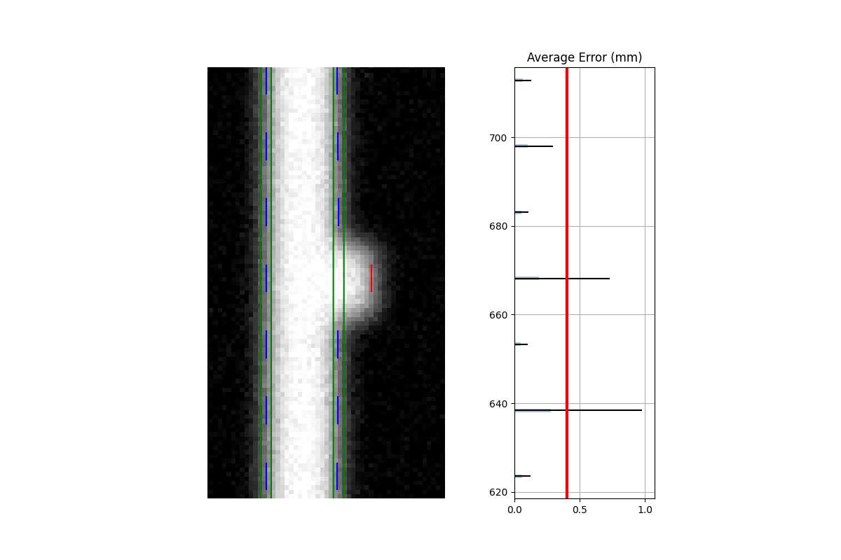
Separate analysis#

Assuming the opposite leaf has no error (see other issues below), the error of a combined analysis is half of the error of the leaf. Over against the argument that it is important to test each leaf, the simple answer is that using a tolerance of half the acceptable error will catch this. I.e. a tolerance of 0.1mm will catch an erroneous leaf up of 0.2mm or more.
Both leaves offset (unilateral): When both leaves are offset to one side.

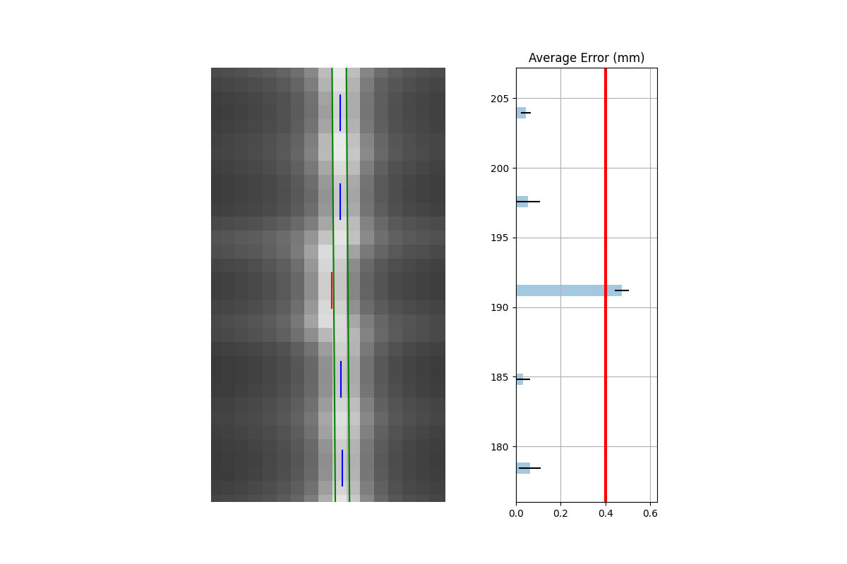
Combined analysis#

Separate analysis with the same tolerance#

As the images show, both analyses detect the problem. This makes sense given that the error was the same direction for both leaves.
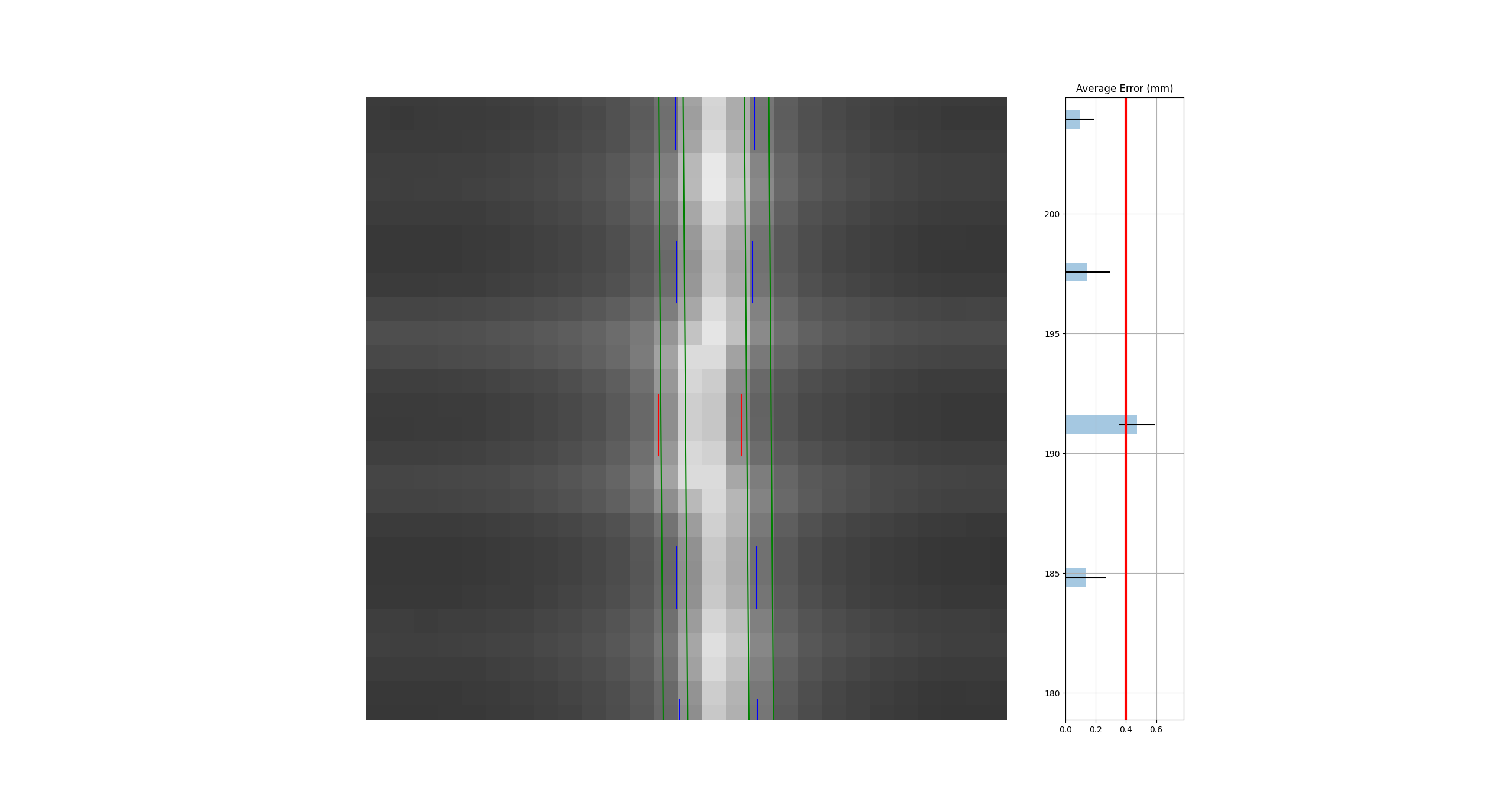
Both leaves offset (mirrored): When both leaves have an offset error, but in opposite directions. This is the only drawback to the combined method.

Combined analysis#

Separate analysis#

Clearly, the separate analysis is advantageous here in terms of detecting the error. The chance of MLC leaves being off by the same amount in opposite directions seems extraordinarily rare. The more likely error would be that the picket width for all leaves is too wide or too narrow. Such a scenario would be easily caught with a DLG test.

To be clear, I’m not against individual leaf analysis, but my anecdotal experience leans toward combined analysis being more robust. Combined with other QA typically performed, I don’t think the medical physics community is all out of whack because they use the combined method vs individual analysis. Use what works for you but realize the strengths of each. Finally, remember that physician contours vary a lot, sometimes by a factor or more. This dwarfs any 0.1mm error of the leaf that we might squabble about. For the scenarios you actually need that 0.1mm, such as SRS, the patient plan QA is the most important factor in determining whether a problem exists.

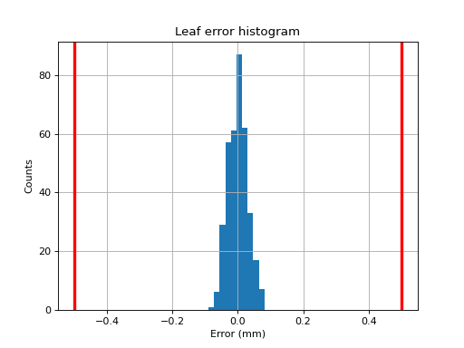
Plotting a histogram#

As of v3.0, you may plot a histogram of the error data like so:

from pylinac import PicketFence
pf = PicketFence.from_demo_image()
pf.analyze()
pf.plot_histogram()

(Source code, png, hires.png, pdf)

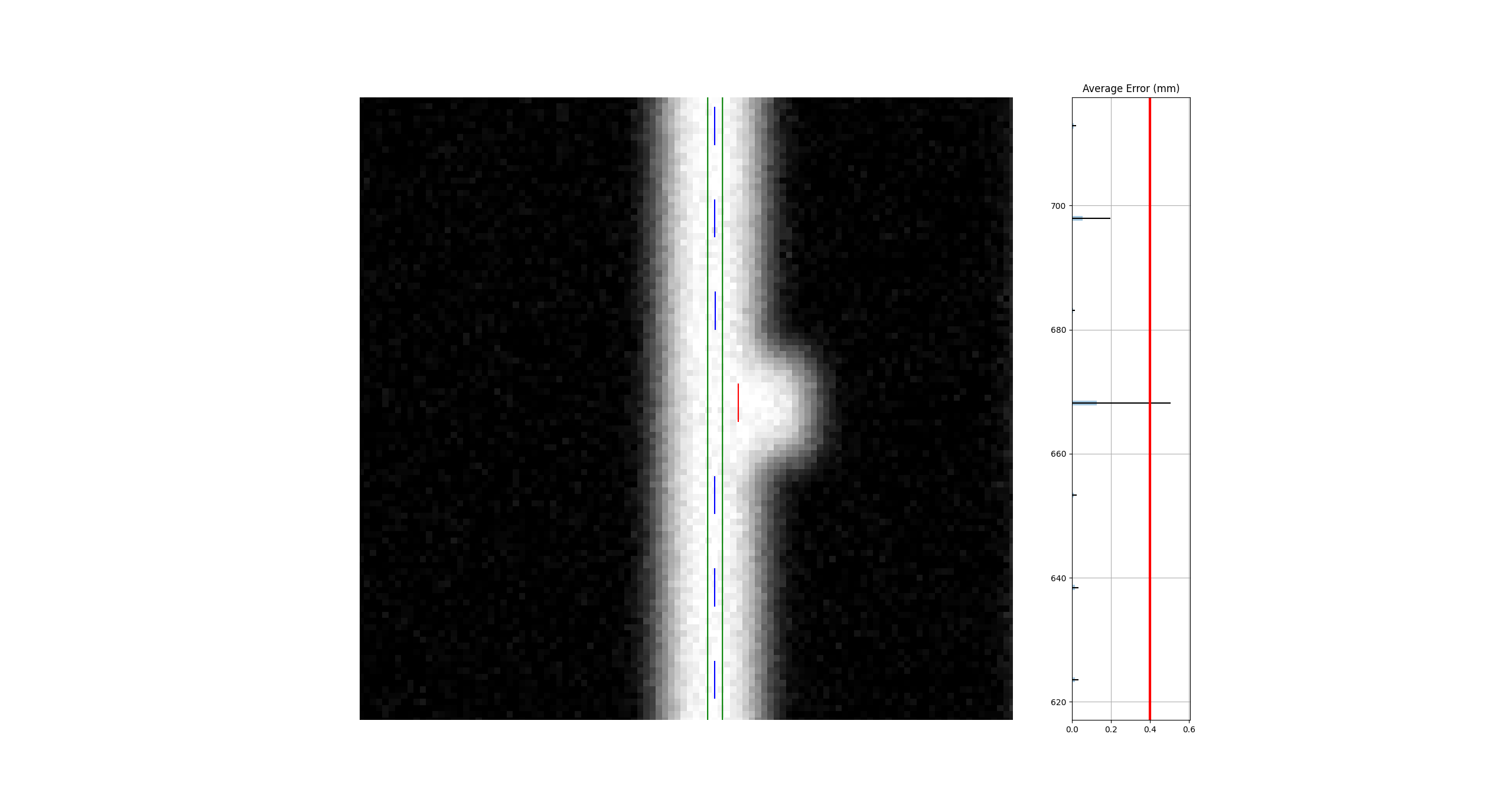
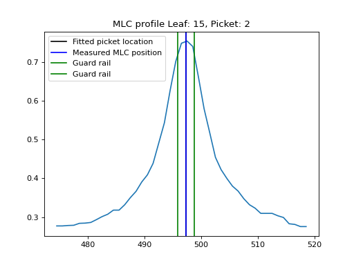
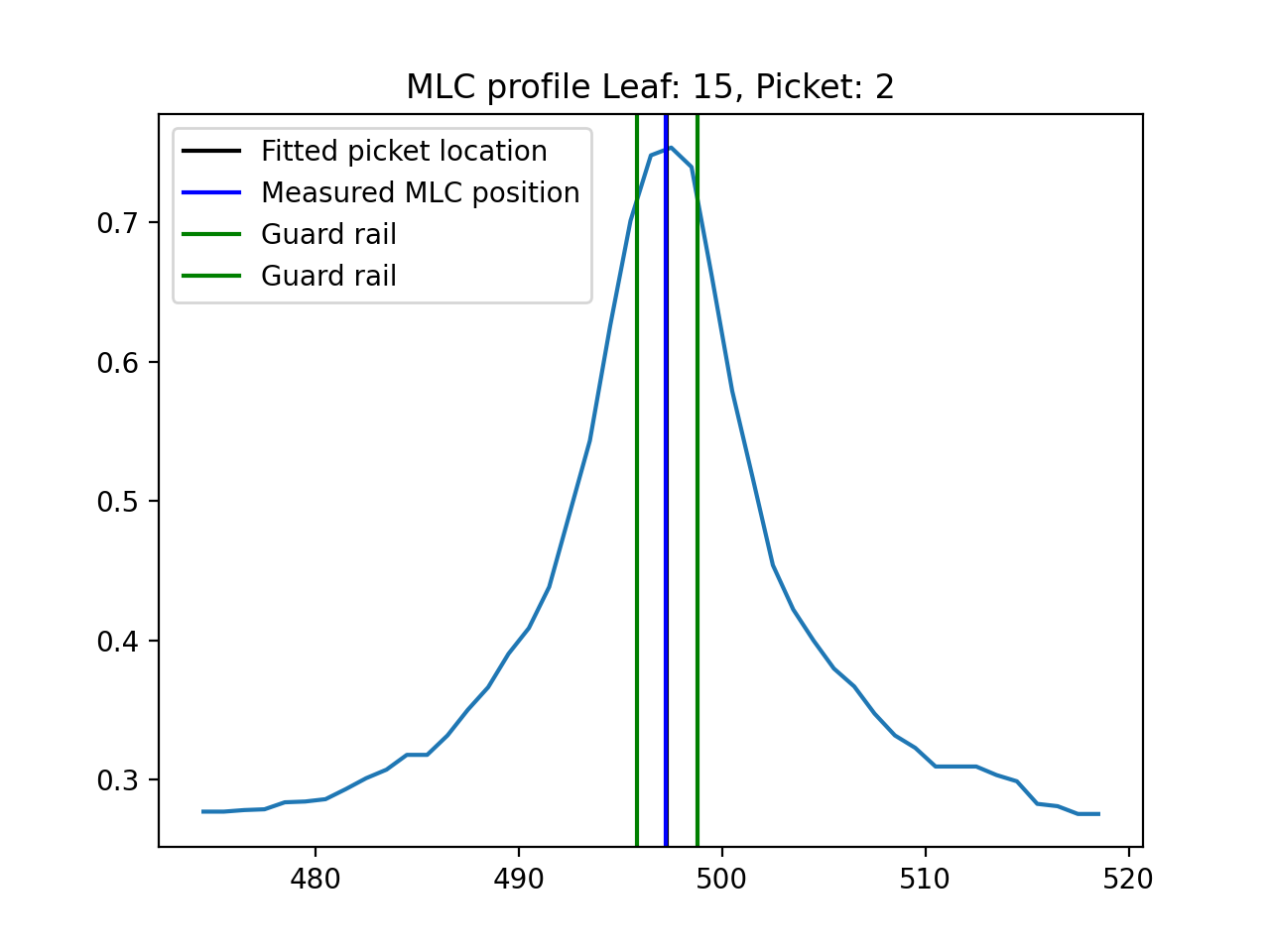
Plotting a leaf profile#

As of v3.0, you may plot an individual leaf profile like so:

from pylinac import PicketFence
pf = PicketFence.from_demo_image()
pf.analyze()
pf.plot_leaf_profile(leaf=15, picket=2)

(Source code, png, hires.png, pdf)

Using a Machine Log#

As of v1.4, you can load a machine log along with your picket fence image. The algorithm will use the expected fluence of the log to determine where the pickets should be instead of fitting to the MLC peaks. Usage looks like this:

from pylinac import PicketFence

pf = PicketFence("my/pf.dcm", log="my/pf_log.bin")
...

Everything else is the same except the measurements are absolute.

Warning

While using a machine log makes the MLC peak error absolute, there may be EPID twist or sag that will exaggerate differences that may or may not be real. Be sure to understand how your imager moves during your picket fence delivery. Even TrueBeams are not immune to EPID twist.

Results will look similar. Here’s an example of the results of using a log:

Customizing MLCs#

As of v2.5, MLC configuration is set a priori (vs empirical determination as before) and the user can also create custom MLC types. Pylinac was only able to handle Millennium and HD Millennium previously.

Preset configurations#

Use a specific preset config:

from pylinac.picketfence import PicketFence, MLC

pf = PicketFence(pf_img, mlc=MLC.MILLENNIUM)

The built-in presets can be seen in attrs of the MLC class.

Creating and using a custom configuration#

Using a custom configuration is very easy. You must create and then pass in a custom MLCArrangement. Leaf arrangements are sets of tuples with the leaf number and leaf width. An example will make this clear:

from pylinac.picketfence import PicketFence, MLCArrangement

# recreate a standard Millennium MLC with 10 leaves of 10mm width, then 40 leaves of 5mm, then 10 of 10mm again.
mlc_setup = MLCArrangement(leaf_arrangement=[(10, 10), (40, 5), (10, 10)])
# add an offset for Halcyon-style or odd-numbered leaf setups
mlc_setup_offset = MLCArrangement(leaf_arrangement=..., offset=2.5)  # offset is in mm

# pass it in to the mlc parameter
pf = PicketFence("path/to/img", mlc=mlc_setup)

# proceed as normal
pf.analyze(...)
...

Acquiring good images#

The following are general tips on getting good images that pylinac will analyze easily. These are in addition to the algorithm allowances and restrictions:

Keep your pickets away from the edges. That is, in the direction parallel to leaf motion keep the pickets at least 1-2cm from the edge.
If you use wide-gap pickets, give a reasonable amount of space between the pickets and keep the gap wider than the picket. I.e. don’t have 5mm spacing between 20mm pickets.
If you use Y-jaws, leave them open 1-2 leaves more than the leaves you want to measure. For example. if you just want to analyze the “central” leaves and set Y-jaws to +/-10cm, the leaves at the edge may not be caught by the algorithm (although see the edge_threshold parameter of analyze). To avoid having to tweak the algorithm, just open the jaws a bit more.
Don’t put anything else in the beam path. This might sound obvious, but I’m continually surprised at the types of images people try to use/take. No, pylinac cannot account for the MV phantom you left on the couch when you took your PF image.
Keep the leaves parallel to an edge. I.e. as close to 0, 90, 270 as possible.

Tips & Tricks#

Use `results_data`#

Using the picketfence module in your own scripts? While the analysis results can be printed out, if you intend on using them elsewhere (e.g. in an API), they can be accessed the easiest by using the analyze() method which returns a PFResult instance.

Note

While the pylinac tooling may change under the hood, this object should remain largely the same and/or expand. Thus, using this is more stable than accessing attrs directly.

Continuing from above:

data = pf.results_data()
data.max_error_mm
data.tolerance_mm
# and more

# return as a dict
data_dict = pf.results_data(as_dict=True)
data_dict["max_error_mm"]
...

EPID sag#

For older linacs, the EPID can also sag at certain angles. Because pylinac assumes a perfect panel, sometimes the analysis will not be centered exactly on the MLC leaves. If you want to correct for this, simply pass the EPID sag in mm:

pf = PicketFence(r"C:/path/saggyPF.dcm")
pf.analyze(sag_adjustment=0.6)

Edge leaves#

For some images, the leaves at the edge of the image or adjacent to the jaws may not be detected. See the image below:

This is caused by the algorithm filtering and can be changed through an analysis parameter. Increase the number to catch more edge leaves:

pf = PicketFence(...)
pf.analyze(..., edge_threshold=3)
...

This results with the edge leaves now being caught in this case. You may need to experiment with this number a few times:

Benchmarking the algorithm#

With the image generator module we can create test images to test the picket fence algorithm on known results. This is useful to isolate what is or isn’t working if the algorithm doesn’t work on a given image and when commissioning pylinac.

Note

Some results here are not perfect. This is because the image generator module cannot necessarily generate pickets of exactly a given gap. The pickets are simulated by setting the pixel values. A gap is rounded to the closest pixel equivalent of the desired gap size; this may not be perfectly symmetric. This affects the error when doing separate leaf analysis and also when evaluating the distance from the CAX. Further, many of these have small amounts of random noise applied on purpose.

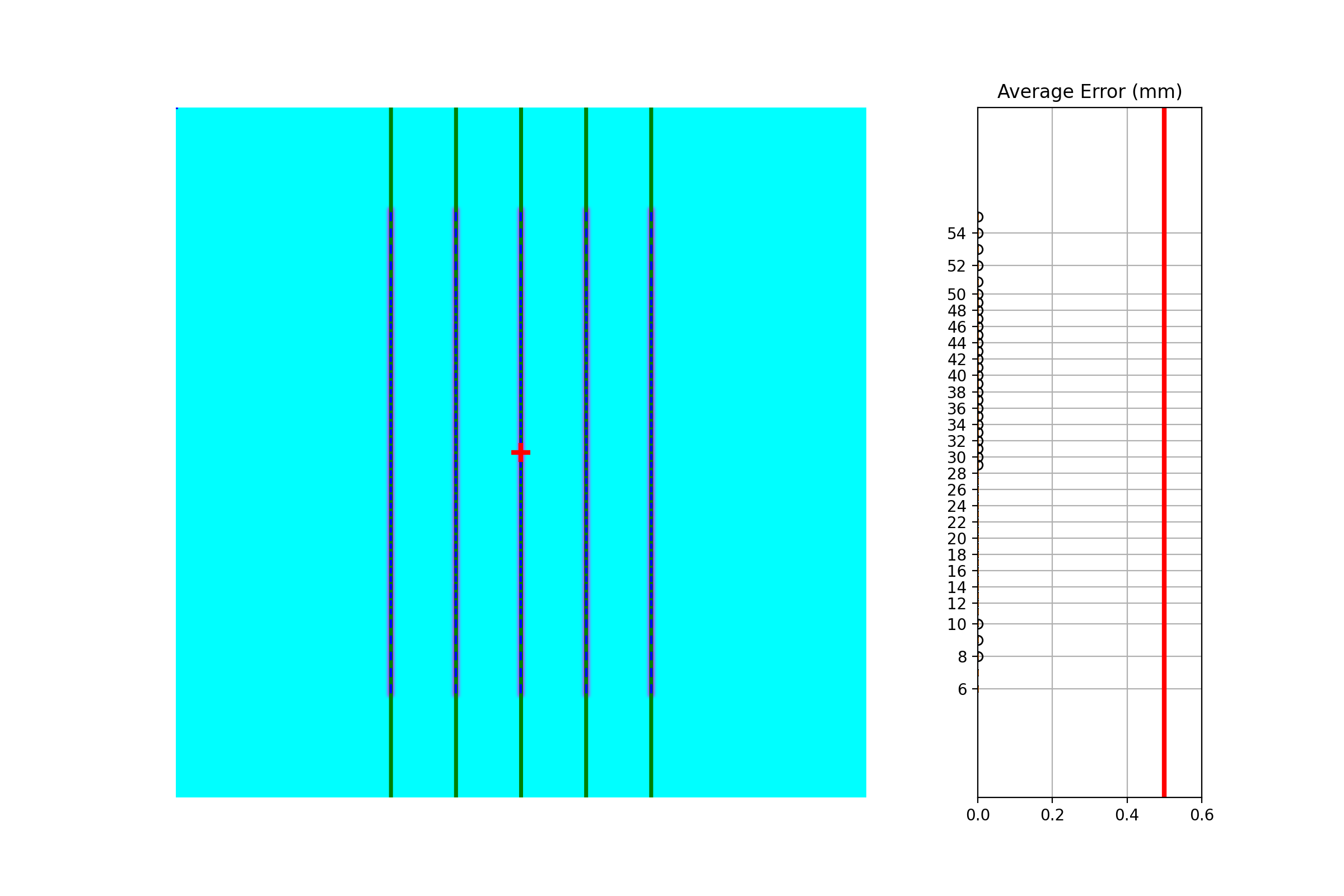
Perfect Up-Down Image#

Below, we generate a DICOM image with slits representing pickets. Several realistic side-effects are not here (such as tongue and groove), but this is perfect for testing. Think of this as the equivalent of measuring a 10x10cm field on the linac vs TPS dose before moving on to VMAT plans.

The script will generate the file, but you can also download it here: perfect_up_down.dcm.

import pylinac
from pylinac.core.image_generator import generate_picketfence, GaussianFilterLayer, PerfectFieldLayer, RandomNoiseLayer, AS1200Image
from pylinac.picketfence import Orientation

# the file name to write the DICOM image to disk to
pf_file = "perfect_.dcm"
# create a PF image with 5 pickets with 40mm spacing between them and 3mm gap. Also applies a gaussian filter to simulate the leaf edges.
generate_picketfence(
    simulator=AS1200Image(sid=1000),
    field_layer=PerfectFieldLayer,
    file_out=pf_file,
    final_layers=[
        GaussianFilterLayer(sigma_mm=1),
    ],
    pickets=5,
    picket_spacing_mm=40,
    picket_width_mm=3,
    orientation=Orientation.UP_DOWN,
)
# load it just like any other
pf = pylinac.PicketFence(pf_file)
pf.analyze(separate_leaves=False, nominal_gap_mm=4)
print(pf.results_data())
pf.plot_analyzed_image()

(Source code, png, hires.png, pdf)

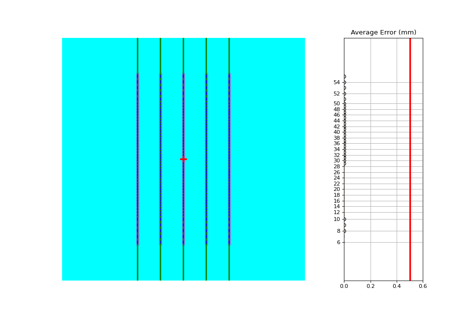
As you can see, the error is zero, the pickets are perfectly straight up and down, and everything looks good.

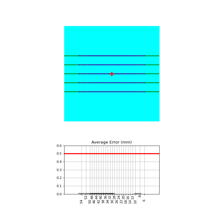
Perfect Left-Right#

Generated file: perfect_left_right.dcm.

import pylinac
from pylinac.core.image_generator import generate_picketfence, GaussianFilterLayer, PerfectFieldLayer, RandomNoiseLayer, AS1200Image
from pylinac.picketfence import Orientation

pf_file = "perfect_left_right.dcm"
generate_picketfence(
    simulator=AS1200Image(sid=1000),
    field_layer=PerfectFieldLayer,
    file_out=pf_file,
    final_layers=[
        GaussianFilterLayer(sigma_mm=1),
    ],
    pickets=5,
    picket_spacing_mm=40,
    picket_width_mm=3,
    orientation=Orientation.LEFT_RIGHT,
)

pf = pylinac.PicketFence(pf_file)
pf.analyze(separate_leaves=False, nominal_gap_mm=4)
print(pf.results_data())
pf.plot_analyzed_image()

(Source code, png, hires.png, pdf)

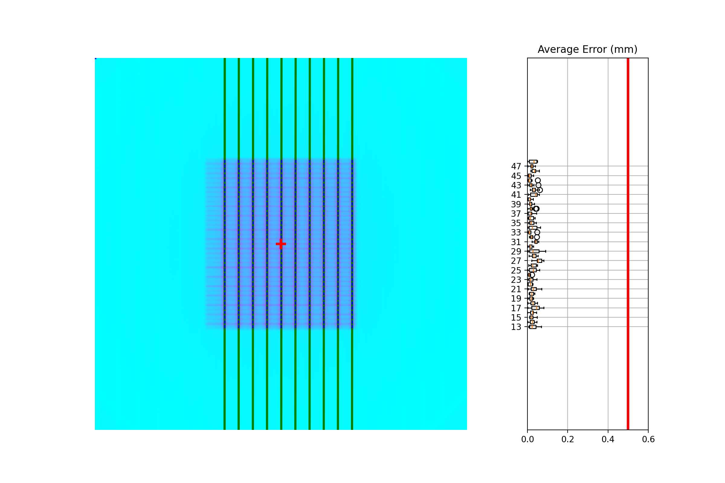
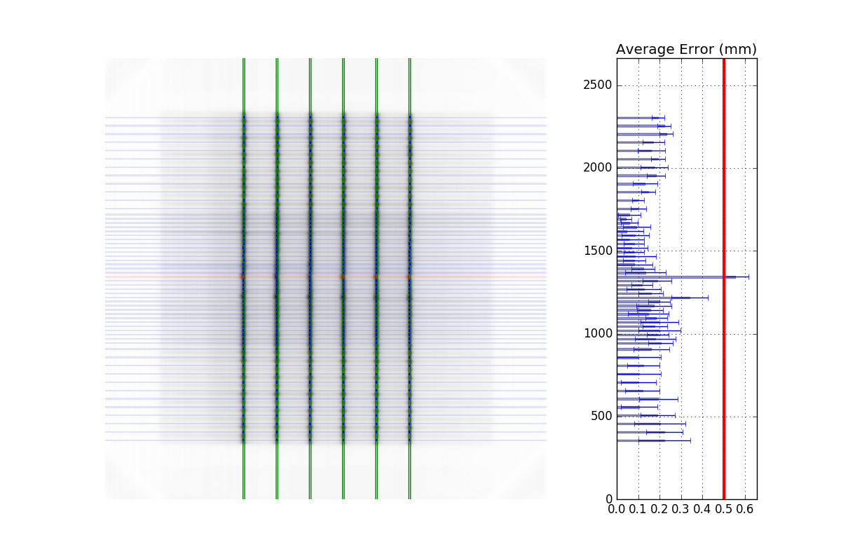
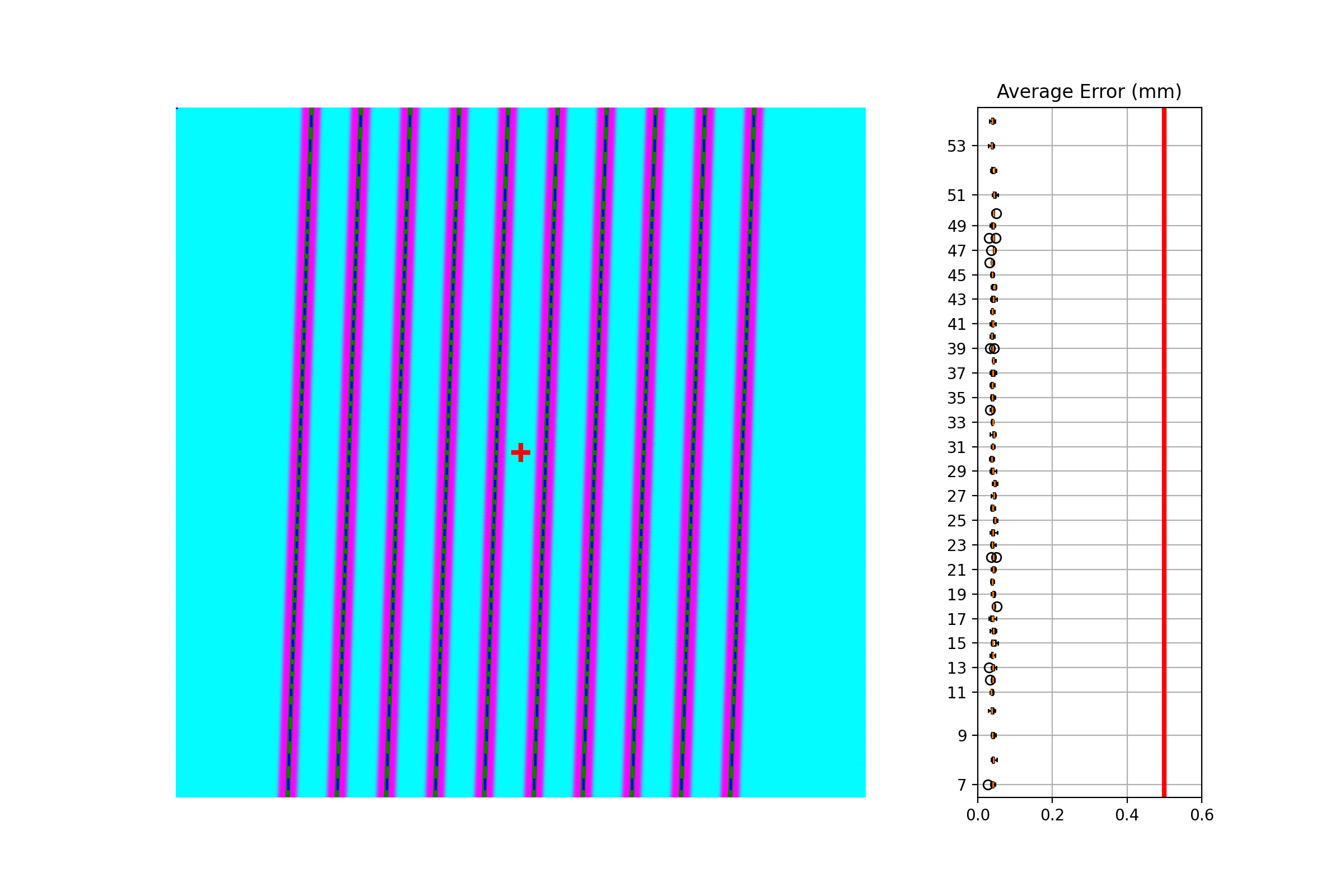
Noisy, Wide-gap Image#

Generated file: noisy_wide_gap_up_down.dcm.

import pylinac
from pylinac.core.image_generator import generate_picketfence, GaussianFilterLayer, PerfectFieldLayer, RandomNoiseLayer, AS1200Image
from pylinac.picketfence import Orientation

pf_file = "noisy_wide_gap_up_down.dcm"
generate_picketfence(
    simulator=AS1200Image(sid=1500),
    field_layer=PerfectFieldLayer,  # this applies a non-uniform intensity about the CAX, simulating the horn effect
    file_out=pf_file,
    final_layers=[
        GaussianFilterLayer(sigma_mm=1),
        RandomNoiseLayer(sigma=0.03)  # add salt & pepper noise
    ],
    pickets=10,
    picket_spacing_mm=20,
    picket_width_mm=10,  # wide-ish gap
    orientation=Orientation.UP_DOWN,
)

pf = pylinac.PicketFence(pf_file)
pf.analyze()
print(pf.results_data())
pf.plot_analyzed_image()

(Source code, png, hires.png, pdf)

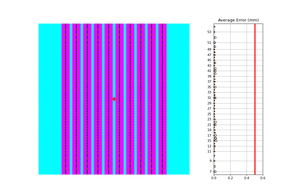
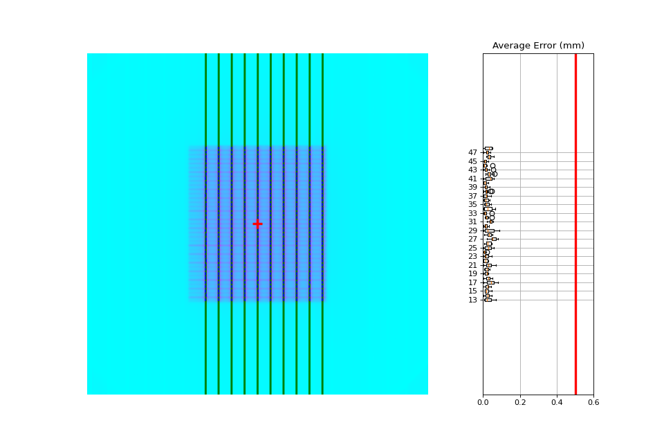
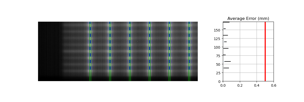
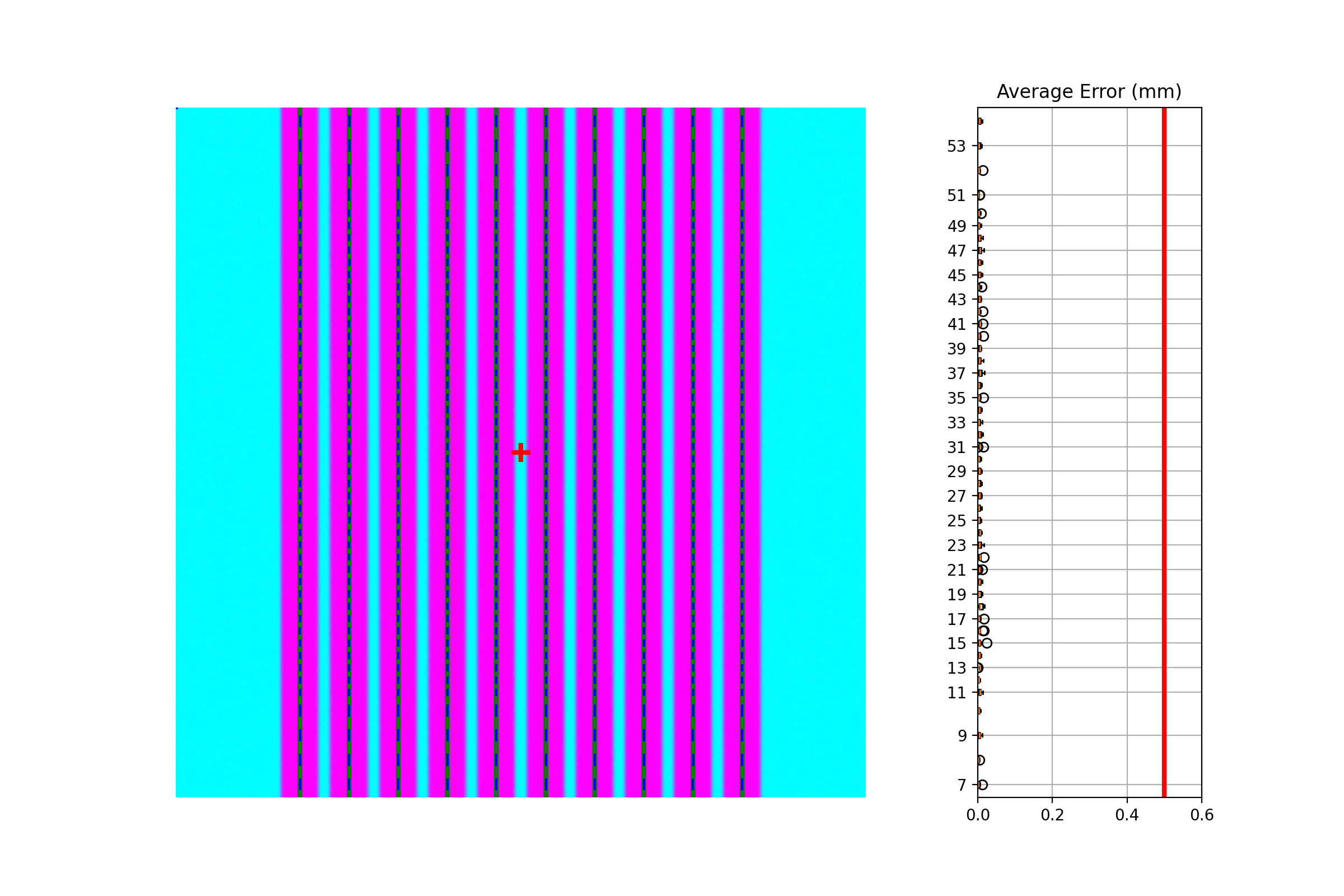
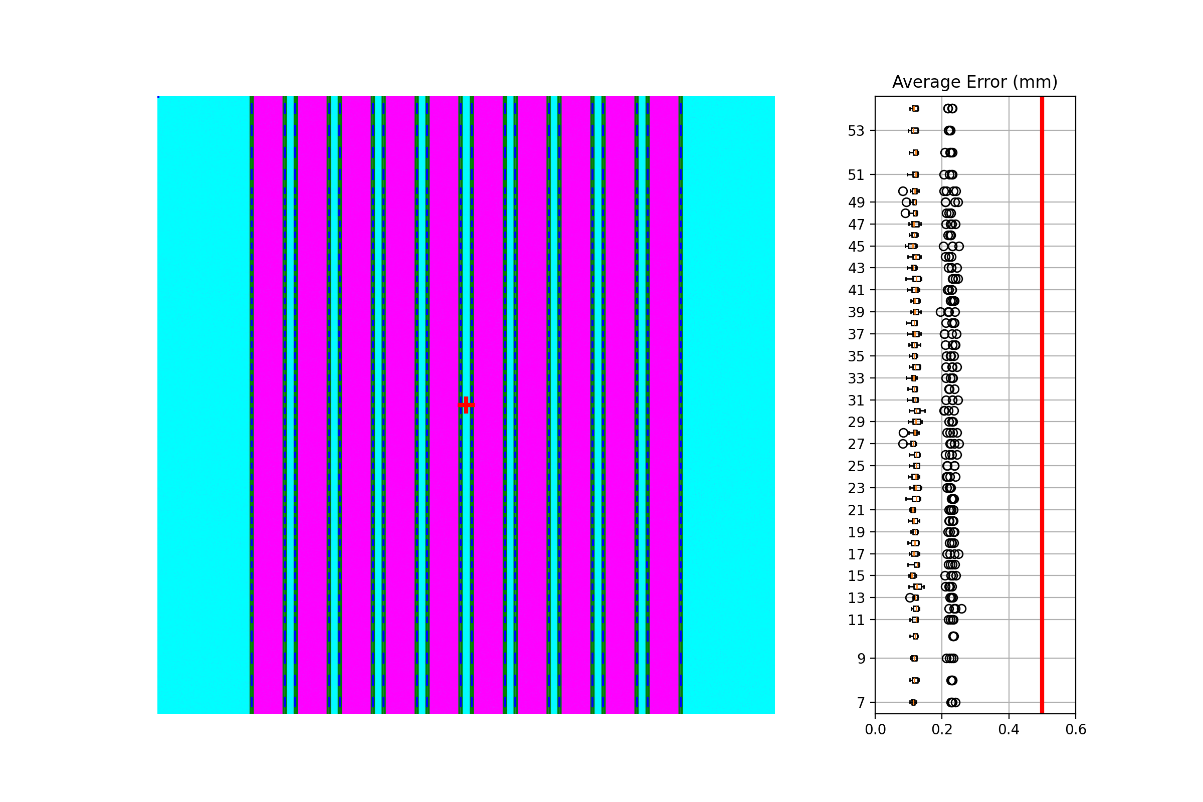
Individual Leaf Analysis#

Let’s now analyze individual leaves using the separate_leaves parameter. This uses the same image base as above; note that the analysis is different.

Generated file: separated_wide_gap_up_down.dcm.

import pylinac
from pylinac.core.image_generator import generate_picketfence, GaussianFilterLayer, PerfectFieldLayer, RandomNoiseLayer, AS1200Image
from pylinac.picketfence import Orientation

pf_file = "separated_wide_gap_up_down.dcm"
generate_picketfence(
    simulator=AS1200Image(sid=1500),
    field_layer=PerfectFieldLayer,  # this applies a non-uniform intensity about the CAX, simulating the horn effect
    file_out=pf_file,
    final_layers=[
        GaussianFilterLayer(sigma_mm=1),
        RandomNoiseLayer(sigma=0.03)  # add salt & pepper noise
    ],
    pickets=10,
    picket_spacing_mm=20,
    picket_width_mm=10,  # wide-ish gap
    orientation=Orientation.UP_DOWN,
)

pf = pylinac.PicketFence(pf_file)
pf.analyze(separate_leaves=True, nominal_gap_mm=10)
print(pf.results())
print(pf.results_data())
pf.plot_analyzed_image()

(Source code, png, hires.png, pdf)

Note that this image has an error of ~0.1mm. This is due to the rounding of pixel values when generating the picket. I.e. it’s not always possible to generate an exactly 10mm gap, but instead is rounded to the nearest pixel equivalent of 10mm.

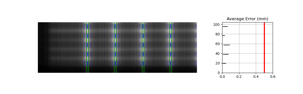
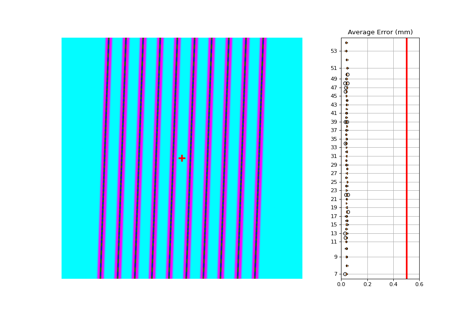
Rotated#

Let’s analyze a slightly rotated image of 2 degrees. Recall that pylinac is limited to ~5 degrees of rotation (depending on picket size).

The image generator doesn’t do the rotation, but is applied later after loading.

Generated file: rotated_up_down.dcm.

from scipy import ndimage

import pylinac
from pylinac.core.image_generator import generate_picketfence, GaussianFilterLayer, PerfectFieldLayer, RandomNoiseLayer, AS1200Image
from pylinac.picketfence import Orientation

pf_file = "rotated_up_down.dcm"
generate_picketfence(
    simulator=AS1200Image(sid=1500),
    field_layer=PerfectFieldLayer,  # this applies a non-uniform intensity about the CAX, simulating the horn effect
    file_out=pf_file,
    final_layers=[
        GaussianFilterLayer(sigma_mm=1),
        RandomNoiseLayer(sigma=0.01)  # add salt & pepper noise
    ],
    pickets=10,
    picket_spacing_mm=20,
    picket_width_mm=5,
    orientation=Orientation.UP_DOWN,
)

pf = pylinac.PicketFence(pf_file)
# here's where we rotate
pf.image.array = ndimage.rotate(pf.image, -2, reshape=False, mode='nearest')
pf.analyze(separate_leaves=False, nominal_gap_mm=5)
print(pf.results())
print(pf.results_data())
pf.plot_analyzed_image()

(Source code, png, hires.png, pdf)

Offset pickets#

In this example, we offset the pickets to simulate an error where the picket was delivered at the wrong x-distance. Lots of physicists cite this as a possibility (or expect their QA software to catch it) but I’ve never seen it. If you have let me know!

Generated file: offset_picket.dcm.

import pylinac
from pylinac.core.image_generator import generate_picketfence, GaussianFilterLayer, PerfectFieldLayer, RandomNoiseLayer, AS1200Image
from pylinac.picketfence import Orientation

pf_file = "offsetpicket.dcm"
generate_picketfence(
    simulator=AS1200Image(sid=1500),
    field_layer=PerfectFieldLayer,  # this applies a non-uniform intensity about the CAX, simulating the horn effect
    file_out=pf_file,
    final_layers=[
        GaussianFilterLayer(sigma_mm=1),
        RandomNoiseLayer(sigma=0.01)  # add salt & pepper noise
    ],
    pickets=5,
    picket_spacing_mm=20,
    picket_width_mm=5,
    picket_offset_error=[-5, 0, 0, 2, 0],  # array of errors; length must match the number of pickets
    orientation=Orientation.UP_DOWN,
)

pf = pylinac.PicketFence(pf_file)
pf.analyze()
print(pf.results())
print(pf.results_data())
pf.plot_analyzed_image()

(Source code, png, hires.png, pdf)

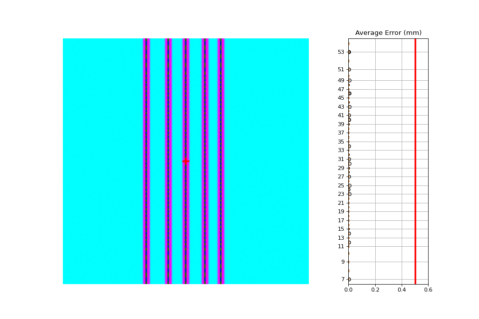
Which produces the following output:

...
Picket offsets from CAX (mm): 45.0 19.9 0.0 -22.0 -40.1
...

The results still show passing. However, note the printed picket offsets from the CAX. The first picket is off by 5mm and the 4th is off by 2mm (as we introduced).

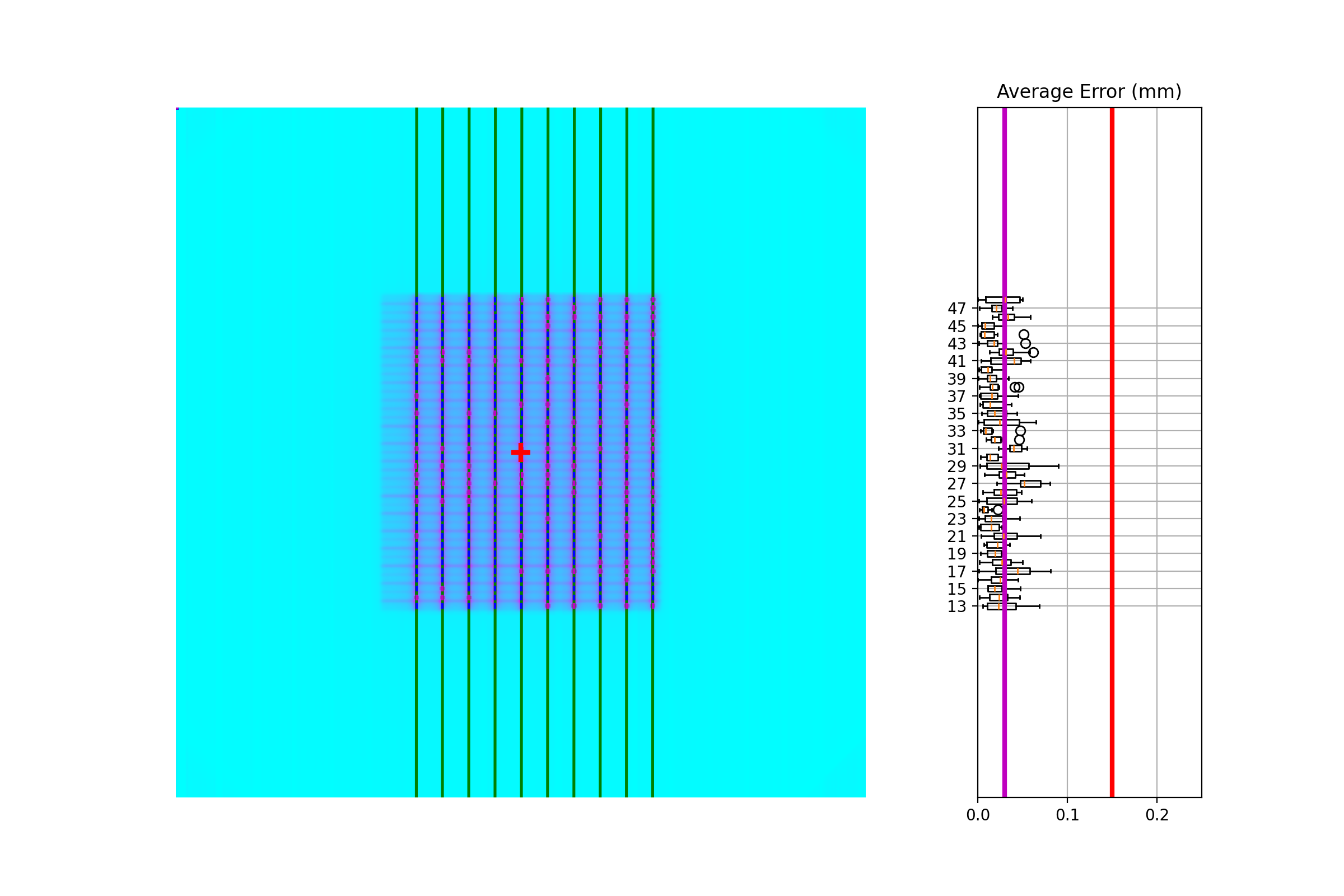
Erroneous leaves#

In this example we introduce errors simulating leaves opening farther than they should.

Generated file: erroneous_leaves.dcm.

import pylinac
from pylinac.core.image_generator import generate_picketfence, GaussianFilterLayer, PerfectFieldLayer, RandomNoiseLayer, AS1200Image
from pylinac.picketfence import Orientation

pf_file = "erroneous_leaves.dcm"
generate_picketfence(
        simulator=AS1200Image(sid=1000),
        field_layer=PerfectFieldLayer,  # this applies a non-uniform intensity about the CAX, simulating the horn effect
        file_out=pf_file,
        final_layers=[
            PerfectFieldLayer(field_size_mm=(5, 10), cax_offset_mm=(2.5, 90)),  # a 10mm gap centered over the picket
            PerfectFieldLayer(field_size_mm=(5, 5), cax_offset_mm=(12.5, -87.5)),  # a 2.5mm extra opening of one leaf
            PerfectFieldLayer(field_size_mm=(5, 5), cax_offset_mm=(22.5, -49)),  # a 1mm extra opening of one leaf
            GaussianFilterLayer(sigma_mm=1),
            RandomNoiseLayer(sigma=0.03)  # add salt & pepper noise
        ],
        pickets=10,
        picket_spacing_mm=20,
        picket_width_mm=5,  # wide-ish gap
        orientation=Orientation.UP_DOWN,
)

pf = pylinac.PicketFence(pf_file)
pf.analyze(separate_leaves=True, nominal_gap_mm=5)
print(pf.results())
print(pf.results_data())
pf.plot_analyzed_image()

(Source code, png, hires.png, pdf)

Algorithm#

The picket fence algorithm uses expected lateral positions of the MLCs and samples those regions for the center of the FWHM to determine the MLC positions:

Allowances

The image can be any size.
Various leaf sizes can be analyzed (e.g. 5 and 10mm leaves for standard Millennium).
Any MLC can be analyzed. See Customizing MLCs
The image can be either orientation (pickets going up-down or left-right).
The image can be at any SSD.
Any EPID type can be used (aS500, aS1000, aS1200).
The EPID panel can have an x or y offset (i.e. translation).

Restrictions

Warning

Analysis can fail or give unreliable results if any Restriction is violated.

The image must be a DICOM image acquired via the EPID.
The delivery must be parallel or nearly-parallel (<~5°) to an image edge; i.e. the collimator should be at 0, 90, or 270 degrees.

Pre-Analysis

Check for noise – Dead pixels can cause wild values in an otherwise well-behaved image. These values can disrupt analysis, but pylinac will try to detect the presence of noise and will apply a median filter if detected.
Check image inversion – Upon loading, the image is sampled near all 4 corners for pixel values. If it is greater than the mean pixel value of the entire image the image is inverted.
Determine orientation – The image is summed along each axis. Pixel percentile values of each axis sum are sampled. The axis with a greater difference in percentile values is chosen as the orientation (The picket axis, it is argued, will have more pixel value variation than the axis parallel to leaf motion.)
Adjust for EPID sag – If a nonzero value is passed for the sag adjustment, the image is shifted along the axis of the pickets; i.e. a +1 mm adjustment for an Up-Down picket image will move expected MLC positions up 1 mm.

Analysis

Find the pickets – The mean profile of the image perpendicular to the MLC travel direction is taken. Major peaks are assumed to be pickets.
Find FWHM at each MLC position – For each picket, a sample of the image in the MLC travel direction is taken at each MLC position. The center of the FWHM of the picket for that MLC position is recorded.
Fit the picket to the positions & calculate error – Once all the MLC positions are determined, the positions from each peak of a picket are fitted to a 1D polynomial which is considered the ideal picket. Differences of each MLC position to the picket polynomial fit at that position are determined, which is the error. When plotted, errors are tested against the tolerance and action tolerance as appropriate.

Troubleshooting#

First, check the general Troubleshooting section. Specific to the picket fence analysis, there are a few things you can do.

Set the image inversion - If you get an error like this: ValueError: max() arg is an empty sequence, one issue may be that the image has the wrong inversion (negative values are positive, etc). Set the analyze flag invert to True to invert the image from the automatic detection. Additionally, if you’re using wide pickets, the image inversion could be wrong. If the pickets are wider than the “valleys” between the pickets this will almost always result in a wrong inversion.
Crop the edges - This is far and away the most common problem. Elekta is notorious for having noisy/bad edges. Pass a larger value into the constructor:
```
pf = PicketFence(..., crop_mm=7)
```
Apply a filter upon load - While pylinac tries to correct for unreasonable noise in the image before analysis, there may still be noise that causes analysis to fail. A way to check this is by applying a median filter upon loading the image:
```
pf = PicketFence("mypf.dcm", filter=5)  # vary the filter size depending on the image
```
Then try performing the analysis.
Check for streak artifacts - It is possible in certain scenarios (e.g. TrueBeam dosimetry mode) to have noteworthy artifacts in the image like so:

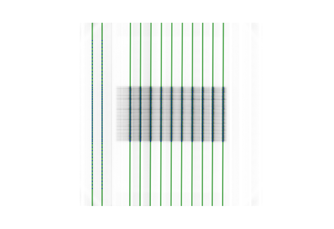
If the artifacts are in the same direction as the pickets then it is possible pylinac is tripping on these artifacts. You can reacquire the image in another mode or simply try again in the same mode. You may also try cropping the image to exclude the artifact:
```
pf = PicketFence("mypf.dcm")
pf.image.array = mypf.image.array[200:400, 150:450]  # or whatever values you want
```
Set the number of pickets - If pylinac is catching too many pickets you can set the number of pickets to find with analyze().
Crop the image - For Elekta images, the 0th column is often an extreme value. For any Elekta image, it is suggested to crop the image. You can crop the image like so:
```
pf = PicketFence(r"my/pf.dcm")
pf.image.crop(pixels=3)
pf.analyze()
...
```

API Documentation#

Main classes#

These are the classes a typical user may interface with.

Bases: ResultsDataMixin[PFResult]

A class used for analyzing EPID images where radiation strips have been formed by the MLCs. The strips are assumed to be parallel to one another and normal to the image edge; i.e. a “left-right” or “up-down” orientation is assumed. Further work could follow up by accounting for any angle.

Parameters#

filename: Name of the file as a string or a file-like object.
filter: If None (default), no filtering will be done to the image. If an int, will perform median filtering over image of size filter.
log: Path to a log file corresponding to the delivery. The expected fluence of the log file is used to construct the pickets. MLC peaks are then compared to an absolute reference instead of a fitted picket.
use_filename: If False (default), no action will be performed. If True, the filename will be searched for keywords that describe the gantry and/or collimator angle. For example, if set to True and the file name was “PF_gantry45.dcm” the gantry would be interpreted as being at 45 degrees.
mlc: The MLC model of the image. Must be an option from the enum MLCs or an MLCArrangement.
crop_mm: The number of mm to crop from all edges. Elekta is infamous for having columns of dead pixels on the side of their images. These need to be cleaned up first. For Varian images, this really shouldn’t make a difference unless the pickets are very close to the edge. Generally speaking, they shouldn’t be for the best accuracy.

leaf_analysis_width: float#

mlc_meas: list#

pickets: list#

tolerance: float#

action_tolerance: float#

image: PFDicomImage#

classmethod from_url(url: str, filter: int = None, image_kwargs: dict | None = None)[source]#: Instantiate from a URL.

classmethod from_demo_image(filter: int = None)[source]#: Construct a PicketFence instance using the demo image.

classmethod from_multiple_images(path_list: Iterable[str | Path], stretch_each: bool = True, method: str = 'mean', mlc: MLC | MLCArrangement | str = MLC.MILLENNIUM, **kwargs)[source]#

Load and superimpose multiple images and instantiate a PF object.

Parameters#

path_listiterable: An iterable of path locations to the files to be loaded/combined.
stretch_eachbool: Whether to stretch each image individually before combining. See load_multiples.
method{‘sum’, ‘mean’}: The method to combine the images. See load_multiples.
mlcMLC, MLCArrangement, or str: The MLC model of the image. Must be an option from the enum MLCs or an MLCArrangement.
kwargs: Passed to load_multiples() and to the PicketFence constructor.

classmethod from_bb_setup(*args, bb_image: str | Path | BinaryIO, bb_diameter: float, **kwargs)[source]#

Construct a PicketFence instance using a BB setup image to find the CAX first. The CAX of the PF image is then overridden w/ the BB location from the first image.

Thank the French for this.

property passed: bool#: Boolean specifying if all MLC positions were within tolerance.

property percent_passing: float#: Return the percentage of MLC positions under tolerance.

property max_error: float#: Return the maximum error found.

property max_error_picket: int#: Return the picket number where the maximum error occurred.

picket_width_stat(picket: int, metric: str = 'max') → float[source]#

Get the statistic of the picket width for the given picket.

Parameters#

picket: The picket number to analyze.
metric: The metric to use. One of ‘max’, ‘median’, ‘mean’, ‘min’.

property max_error_leaf: int | str#: Return the leaf/leaf pair that had the maximum error. This will be a single int value (i.e. either/both A and B) for classic analysis or a fully-qualified name for separate analysis. E.g. A43

failed_leaves() → list[int] | list[str][source]#: A list of the failed leaves. Either the leaf number or the bank+leaf number if using separate leaves.

property abs_median_error: float#: Return the median error found.

property num_pickets: int#: Return the number of pickets determined.

property mean_picket_spacing: float#: The average distance between pickets in mm.

plot_leaf_profile(leaf: str | int, picket: int, show: bool = True)[source]#

Plot the leaf profile of a given leaf pair parallel to leaf motion.

Parameters#

leaf: The leaf to plot. If separate_leaves is True, this will be a string like “A15” or “B33”. If separate_leaves is False, this must be an int, like 15 or 33.
picket: An int of the picket number. Pickets start from the 0-side of an image. E.g. for left-right PFs, this would start on the left; for up-down this would start at the bottom.

save_leaf_profile(filename: str | Path | BinaryIO, leaf: str | int, picket: int, **kwargs)[source]#: Save the leaf profile plot to disk or stream. See plot_leaf_profile for parameter hints. Kwargs are passed to matplotlib.savefig()

static run_demo(tolerance: float = 0.5, action_tolerance: float = None) → None[source]#: Run the Picket Fence demo using the demo image. See analyze() for parameter info.

analyze(tolerance: float = 0.5, action_tolerance: float | None = None, num_pickets: int | None = None, sag_adjustment: float | int = 0, orientation: Orientation | str | None = None, invert: bool = False, leaf_analysis_width_ratio: float = 0.4, picket_spacing: float | None = None, height_threshold: float = 0.5, edge_threshold: float = 1.5, peak_sort: str = 'peak_heights', required_prominence: float = 0.2, fwxm: int = 50, separate_leaves: bool = False, nominal_gap_mm: float = 3, central_axis: Point | None = None) → None[source]#

Analyze the picket fence image.

Parameters#

tolerance: The tolerance of difference in mm between an MLC pair position and the picket fit line.
action_tolerance: If None (default), no action tolerance is set or compared to. If an int or float, the MLC pair measurement is also compared to this tolerance. Must be lower than tolerance. This value is usually meant to indicate that a physicist should take an “action” to reduce the error, but should not stop treatment.
num_pickets: The number of pickets in the image. A helper parameter to limit the total number of pickets, only needed if analysis is catching more pickets than there really are.
sag_adjustment: The amount of shift in mm to apply to the image to correct for EPID sag. For Up-Down picket images, positive moves the image down, negative up. For Left-Right picket images, positive moves the image left, negative right.
orientation: If None (default), the orientation is automatically determined. If for some reason the determined orientation is not correct, you can pass it directly using this parameter. If passed a string with ‘u’ (e.g. ‘up-down’, ‘u-d’, ‘up’) it will set the orientation of the pickets as going up-down. If passed a string with ‘l’ (e.g. ‘left-right’, ‘lr’, ‘left’) it will set it as going left-right.
invert: If False (default), the inversion of the image is automatically detected and used. If True, the image inversion is reversed from the automatic detection. This is useful when runtime errors are encountered.
leaf_analysis_width_ratio: The ratio of the leaf width to use as part of the evaluation. E.g. if the ratio is 0.5, the center half of the leaf will be used. This helps avoid tongue and groove influence.
picket_spacing: If None (default), the spacing between pickets is determined automatically. If given, it should be an int or float specifying the number of PIXELS apart the pickets are.
height_threshold: The threshold that the MLC peak needs to be above to be considered a picket (vs background). Lower if not all leaves are being caught. Note that for FFF beams this would very likely need to be lowered.
edge_threshold: The threshold of pixel value standard deviation within the analysis window of the MLC leaf to be considered a full leaf. This is how pylinac removes MLCs that are eclipsed by the jaw. This also is how to omit or catch leaves at the edge of the field. Raise to catch more edge leaves.
peak_sort: Either ‘peak_heights’ or ‘prominences’. This is the method for determining the peaks. Usually not needed unless the wrong number of pickets have been detected. See the scipy.signal.find_peaks function for more information.
required_prominence: The required height of the picket (not individual MLCs) to be considered a peak. Pylinac takes a mean of the image axis perpendicular to the leaf motion to get an initial guess of the peak locations and also to determine picket spacing. Changing this can be useful for wide-gap tests where the shape of the beam horns can form two or more local maximums in the picket area. Increase if for wide-gap images that are catching too many pickets. Consider lowering for FFF beams if there are analysis issues.

Warning

We do not recommend performing FFF wide-gap PF tests. Make your FFF pickets narrow or measure with a flat beam instead.
fwxm: For each MLC kiss, the profile is a curve from low to high to low. The FWXM (0-100) is the height to use to measure to determine the center of the curve, which is the surrogate for MLC kiss position. I.e. for each MLC kiss, what height of the picket should you use to actually determine the center location? It is unusual to change this. If you have something in the way (we’ve seen crazy examples with a BB in the way) you may want to increase this.
separate_leaves: Whether to analyze leaves individually (each tip) or as a set (combined, center of the picket). False is the default for backwards compatibility.
nominal_gap_mm: The expected gap of the pickets in mm. Only used when separate leaves is True. Due to the DLG and EPID scattering, this value will have to be determined by you with a known good delivery.
central_axis: The central axis of the beam. If None (default), the CAX is automatically determined. This is used for French regulations where the CAX is set to the BB location from a separate image.

plot_analyzed_image(guard_rails: bool = True, mlc_peaks: bool = True, overlay: bool = True, leaf_error_subplot: bool = True, show: bool = True, figure_size: str | tuple = 'auto') → None[source]#

Plot the analyzed image.

Parameters#

guard_rails: Do/don’t plot the picket “guard rails” around the ideal picket
mlc_peaks: Do/don’t plot the detected MLC peak positions.
overlay: Do/don’t plot the alpha overlay of the leaf status.
leaf_error_subplot: If True, plots a linked leaf error subplot adjacent to the PF image plotting the average and standard deviation of leaf error.
show: Whether to display the plot. Set to false for saving to a figure, etc.
figure_size: Either ‘auto’ or a tuple. If auto, the figure size is set depending on the orientation. If a tuple, this is the figure size to use.

save_analyzed_image(filename: str | BytesIO, guard_rails: bool = True, mlc_peaks: bool = True, overlay: bool = True, leaf_error_subplot: bool = False, **kwargs) → None[source]#: Save the analyzed figure to a file. See plot_analyzed_image() for further parameter info.

results(as_list: bool = False) → str[source]#: Return results of analysis. Use with print().

publish_pdf(filename: str | BytesIO, notes: str = None, open_file: bool = False, metadata: dict = None, bins: int = 10, logo: Path | str | None = None) → None[source]#

Publish (print) a PDF containing the analysis, images, and quantitative results.

Parameters#

filename(str, file-like object}: The file to write the results to.
notesstr, list of strings: Text; if str, prints single line. If list of strings, each list item is printed on its own line.
open_filebool: Whether to open the file using the default program after creation.
metadatadict: Extra data to be passed and shown in the PDF. The key and value will be shown with a colon. E.g. passing {‘Author’: ‘James’, ‘Unit’: ‘TrueBeam’} would result in text in the PDF like: ————– Author: James Unit: TrueBeam ————–
bins: int: Number of bins to show for the histogram
logo: Path, str: A custom logo to use in the PDF report. If nothing is passed, the default pylinac logo is used.

mlc_skew() → float[source]#: Apparent rotation in degrees of the MLC. This could be conflated with the EPID skew, so be careful when interpreting this value.

plot_histogram(bins: int = 10, show: bool = True) → None[source]#: Plot a histogram of the leaf errors

save_histogram(filename: [<class 'str'>, <class 'pathlib.Path'>, <class 'typing.BinaryIO'>], bins: int = 10, **kwargs) → None[source]#: Save a histogram of the leaf errors

property orientation: Orientation#: The orientation of the image, either Up-Down or Left-Right.

class pylinac.picketfence.MLCArrangement(leaf_arrangement: list[tuple[int, float]], offset: float = 0)[source]#

Bases: object

Construct an MLC array

Parameters#

leaf_arrangement: Description of the leaf arrangement. List of tuples containing the number of leaves and leaf width. E.g. (10, 5) is 10 leaves with 5mm widths.
offset: The offset in mm of the leaves. Used for asymmetric arrangements. E.g. -2.5mm will shift the arrangement 2.5mm to the left.

property leaves: list[int]#: The leaf numbers; index pairs with the centers. Assumes that the first leaf center is toward the target and the last leaf center is towards the gun.

class pylinac.picketfence.Orientation(value, names=None, *, module=None, qualname=None, type=None, start=1, boundary=None)[source]#

Bases: Enum

Possible orientations of the image

UP_DOWN = 'Up-Down'#

LEFT_RIGHT = 'Left-Right'#

class pylinac.picketfence.MLC(value, names=None, *, module=None, qualname=None, type=None, start=1, boundary=None)[source]#

Bases: Enum

The pre-built MLC types

MILLENNIUM = {'arrangement': <pylinac.picketfence.MLCArrangement object>, 'name': 'Millennium'}#

HD_MILLENNIUM = {'arrangement': <pylinac.picketfence.MLCArrangement object>, 'name': 'HD Millennium'}#

BMOD = {'arrangement': <pylinac.picketfence.MLCArrangement object>, 'name': 'B Mod'}#

AGILITY = {'arrangement': <pylinac.picketfence.MLCArrangement object>, 'name': 'Agility'}#

MLCI = {'arrangement': <pylinac.picketfence.MLCArrangement object>, 'name': 'MLCi'}#

HALCYON_DISTAL = {'arrangement': <pylinac.picketfence.MLCArrangement object>, 'name': 'Halcyon distal'}#

HALCYON_PROXIMAL = {'arrangement': <pylinac.picketfence.MLCArrangement object>, 'name': 'Halcyon proximal'}#

class pylinac.picketfence.PFResult(*, pylinac_version: str = '3.22.0', date_of_analysis: datetime = None, tolerance_mm: float, action_tolerance_mm: float | None, percent_leaves_passing: float, number_of_pickets: int, absolute_median_error_mm: float, max_error_mm: float, max_error_picket: int, max_error_leaf: str | int, mean_picket_spacing_mm: float, offsets_from_cax_mm: list[float], passed: bool, failed_leaves: list[str] | list[int], mlc_skew: float, picket_widths: dict[str, dict[str, float]])[source]#

Bases: ResultBase

This class should not be called directly. It is returned by the results_data() method. It is a dataclass under the hood and thus comes with all the dunder magic.

Use the following attributes as normal class attributes.

Create a new model by parsing and validating input data from keyword arguments.

Raises [ValidationError][pydantic_core.ValidationError] if the input data cannot be validated to form a valid model.

self is explicitly positional-only to allow self as a field name.

tolerance_mm: float#

action_tolerance_mm: float | None#

percent_leaves_passing: float#

number_of_pickets: int#

absolute_median_error_mm: float#

max_error_mm: float#

max_error_picket: int#

max_error_leaf: str | int#

mean_picket_spacing_mm: float#

offsets_from_cax_mm: list[float]#

passed: bool#

failed_leaves: list[str] | list[int]#

mlc_skew: float#

picket_widths: dict[str, dict[str, float]]#

model_computed_fields: ClassVar[dict[str, ComputedFieldInfo]] = {}#: A dictionary of computed field names and their corresponding ComputedFieldInfo objects.

model_config: ClassVar[ConfigDict] = {'arbitrary_types_allowed': True}#: Configuration for the model, should be a dictionary conforming to [ConfigDict][pydantic.config.ConfigDict].

model_fields: ClassVar[dict[str, FieldInfo]] = {'absolute_median_error_mm': FieldInfo(annotation=float, required=True), 'action_tolerance_mm': FieldInfo(annotation=Union[float, NoneType], required=True), 'date_of_analysis': FieldInfo(annotation=datetime, required=False, default_factory=builtin_function_or_method), 'failed_leaves': FieldInfo(annotation=Union[list[str], list[int]], required=True), 'max_error_leaf': FieldInfo(annotation=Union[str, int], required=True), 'max_error_mm': FieldInfo(annotation=float, required=True), 'max_error_picket': FieldInfo(annotation=int, required=True), 'mean_picket_spacing_mm': FieldInfo(annotation=float, required=True), 'mlc_skew': FieldInfo(annotation=float, required=True), 'number_of_pickets': FieldInfo(annotation=int, required=True), 'offsets_from_cax_mm': FieldInfo(annotation=list[float], required=True), 'passed': FieldInfo(annotation=bool, required=True), 'percent_leaves_passing': FieldInfo(annotation=float, required=True), 'picket_widths': FieldInfo(annotation=dict[str, dict[str, float]], required=True), 'pylinac_version': FieldInfo(annotation=str, required=False, default='3.22.0'), 'tolerance_mm': FieldInfo(annotation=float, required=True)}#

Metadata about the fields defined on the model, mapping of field names to [FieldInfo][pydantic.fields.FieldInfo].

This replaces Model.__fields__ from Pydantic V1.

Supporting Classes#

You generally won’t have to interface with these unless you’re doing advanced behavior.

class pylinac.picketfence.PFDicomImage(path: str, **kwargs)[source]#

Bases: LinacDicomImage

A subclass of a DICOM image that checks for noise and inversion when instantiated. Can also adjust for EPID sag.

Parameters#

pathstr, file-object: The path to the file or the data stream.
dtypedtype, None, optional: The data type to cast the image data as. If None, will use whatever raw image format is.
dpiint, float: The dots-per-inch of the image, defined at isocenter.

Note

If a DPI tag is found in the image, that value will override the parameter, otherwise this one will be used.
sidint, float: The Source-to-Image distance in mm.
sadfloat: The Source-to-Axis distance in mm.
raw_pixelsbool: Whether to apply pixel intensity correction to the DICOM data. Typically, Rescale Slope, Rescale Intercept, and other tags are included and meant to be applied to the raw pixel data, which is potentially compressed. If True, no correction will be applied. This is typically used for scenarios when you want to match behavior to older or different software.

adjust_for_sag(sag: int, orientation: str | Orientation) → None[source]#: Roll the image to adjust for EPID sag.

property center: Point#: Override the central axis call in the event we passed it directly

class pylinac.picketfence.Picket(mlc_measurements: list[MLCValue], log_fits, orientation: Orientation, image: PFDicomImage, tolerance: float, separate_leaves: bool, nominal_gap: float)[source]#

Bases: object

Holds picket information in a Picket Fence test.

get_fit() → poly1d[source]#: The fit of a polynomial to the MLC measurements.

skew() → float[source]#: The slope/skew of the picket

property dist2cax: float#: The distance from the CAX to the picket, in mm.

property left_guard_separated: Sequence[poly1d]#: The line representing the left-sided guard rails. When not doing separate analysis, the left and right rails will overlap.

property right_guard_separated#: The line representing the right-sided guard rails.

add_guards_to_axes(axis: Axes, color: str = 'g') → None[source]#: Plot guard rails to the axis.

class pylinac.picketfence.MLCValue(picket_num: int, approx_idx: int, leaf_width: float, leaf_center: float, picket_spacing: float, orientation: Orientation, leaf_analysis_width_ratio: float, tolerance: float, action_tolerance: float | None, leaf_num: int, approx_peak_val: float, image_window: ndarray, image: PFDicomImage, fwxm: int, separate_leaves: bool, nominal_gap_mm: float)[source]#

Bases: object

Representation of an MLC kiss or of each MLC about a kiss.

property full_leaf_nums: Sequence[str | int]#: The fully-qualified leaf names. This will be the simple leaf number for traditional analysis or the bank+leaf num for separate leaves.

plot2axes(axes: Axes, width: float | int = 1) → None[source]#: Plot the measurement to the axes.

property passed: Sequence[bool]#: Whether the MLC kiss or leaf was within tolerance.

property passed_action: Sequence[bool] | None#: Whether the MLC kiss or leaf was within the action tolerance.

property bg_color: Sequence[str]#: The color of the measurement when the PF image is plotted, based on pass/fail status.

property picket_positions: Sequence[float]#: The position(s) of the pickets in mm

property error: Sequence[float]#: The error (difference) of the MLC measurement and the picket fit. If using individual leaf analysis, returns both errors otherwise return one.

property max_abs_error: float#: The maximum absolute error

property marker_lines: list[Line]#: The line(s) representing the MLC measurement position. When using separated leaves there are two lines. Traditional analysis returns one.

plot_overlay2axes(axes) → None[source]#: Create a rectangle overlay with the width of the error. I.e. it stretches from the picket fit to the MLC position. Gives more visual size to the

Picket Fence#

Overview#

Concepts#

Running the Demo#

Acquiring the Image#

Typical Use#

Analyzing individual leaves#

Individual leaf detection vs combined#

Plotting a histogram#

Plotting a leaf profile#

Using a Machine Log#

Customizing MLCs#

Preset configurations#

Creating and using a custom configuration#

Acquiring good images#

Tips & Tricks#

Use results_data#

EPID sag#

Edge leaves#

Benchmarking the algorithm#

Perfect Up-Down Image#

Perfect Left-Right#

Noisy, Wide-gap Image#

Individual Leaf Analysis#

Rotated#

Offset pickets#

Erroneous leaves#

Algorithm#

Troubleshooting#

API Documentation#

Main classes#

Parameters#

Parameters#

Parameters#

Parameters#

Parameters#

Parameters#

Parameters#

Parameters#

Supporting Classes#

Parameters#

Use `results_data`#