Custom Image Metrics#

New in version 3.16.

Pylinac images can now have arbitrary metrics calculated on them, similar to profiles. This can be useful for calculating and finding values and regions of interest in images. The system is quite flexible and allows for any number of metrics to be calculated on an image. Furthermore, this allows for re-usability of metrics, as they can be applied to any image.

Use Cases#

Calculate the mean pixel value of an area of an image.
Finding an object in the image.
Calculating the distance between two objects in an image.

Basic Usage#

To calculate metrics on an image, simply pass the metric(s) to the compute method of the image:

from pylinac.core.image import DicomImage
from pylinac.core.metrics import DiskLocator, DiskRegion

img = DicomImage("my_image.dcm")
metric = img.compute(
    metrics=DiskLocator(
        expected_position=(100, 100),
        search_window=(30, 30),
        radius=10,
        radius_tolerance=2,
    )
)
print(metric)

You may compute multiple metrics by passing a list of metrics:

from pylinac.core.image import DicomImage
from pylinac.core.metrics import DiskLocator, DiskRegion

img = DicomImage("my_image.dcm")
metrics = img.compute(
    metrics=[
        # disk 1
        DiskLocator(
            expected_position=(100, 100),
            search_window=(30, 30),
            radius=10,
            radius_tolerance=2,
        ),
        # disk 2
        DiskLocator(
            expected_position=(200, 200),
            search_window=(30, 30),
            radius=10,
            radius_tolerance=2,
        ),
    ]
)
print(metrics)

Metrics might have something to plot on the image. If so, the plot method of the image will plot the metric(s) on the image:

from pylinac.core.image import DicomImage
from pylinac.core.metrics import DiskLocator, DiskRegion

img = DicomImage("my_image.dcm")
metrics = img.compute(
    metrics=[
        # disk 1
        DiskLocator(
            expected_position=(100, 100),
            search_window=(30, 30),
            radius=10,
            radius_tolerance=2,
        ),
        # disk 2
        DiskLocator(
            expected_position=(200, 200),
            search_window=(30, 30),
            radius=10,
            radius_tolerance=2,
        ),
    ]
)
img.plot()  # plots the image with the BB positions overlaid

Built-in Metrics#

Out of the box, three metrics currently exist: DiskLocator, DiskRegion and GlobalDiskLocator.

These metrics will find disks, usually BBs, in an image and then return the location or region properties.

Single Disk Locators#

Note

The values provided below are in pixels. The following sections show how variants of how to use the metrics using physical units and relative to the center of the image.

Here’s an example of using the DiskLocator:

Search for a disk 100 pixels right and 100 pixels down from the top left of the image#

from pylinac.core.image import DicomImage
from pylinac.core.metrics import DiskLocator, DiskRegion

img = DicomImage("my_image.dcm")
img.compute(
    metrics=[
        DiskLocator(
            expected_position=(100, 100),
            search_window=(30, 30),
            radius=10,
            radius_tolerance=2,
        )
    ]
)
img.plot()

This will search for a disk (BB) in the image at the expected position and window size for a disk of a given radius and tolerance. If the disk is found, the location will be returned as a Point object. If the disk is not found, a ValueError will be raised.

The DiskRegion metric is similar, but instead of returning the location, it returns a scikit-image regionprops object that is the region of the disk. This allows one to then calculate things like the weighted centroid, area, etc.

Using physical units#

While pixels are useful, it is sometimes easier to use physical units.

To perform the same Disk/BB location using mm instead of pixels:

Search for a disk 30mm right and 30mm down from the top left of the image#

from pylinac.core.image import DicomImage
from pylinac.core.metrics import DiskLocator, DiskRegion

img = DicomImage("my_image.dcm")
img.compute(
    metrics=[
        # these are all in mm
        DiskLocator.from_physical(
            expected_position_mm=(30, 30),
            search_window_mm=(10, 10),
            radius_mm=4,
            radius_tolerance_mm=2,
        )
    ]
)
img.plot()

Relative to center#

We can also specify the expected position relative to the center of the image.

Important

We can do this using pixels OR physical units.

This will look for the disk/BB 30 pixels right and 30 pixels down from the center of the image:

Relative to center using pixels#

from pylinac.core.image import DicomImage
from pylinac.core.metrics import DiskLocator, DiskRegion

img = DicomImage("my_image.dcm")
img.compute(
    metrics=[
        # these are all in pixels
        DiskLocator.from_center(
            expected_position=(30, 30),
            search_window=(10, 10),
            radius=4,
            radius_tolerance=2,
        )
    ]
)
img.plot()

This will look for the disk/BB 30mm right and 30mm down from the center of the image:

Relative to center using physical units#

img.compute(
    metrics=[
        # these are all in mm
        DiskLocator.from_center_physical(
            expected_position_mm=(30, 30),
            search_window_mm=(10, 10),
            radius_mm=4,
            radius_tolerance_mm=2,
        )
    ]
)
img.plot()

Global Disk Locator#

New in version 3.17.

The GlobalDiskLocator metric is similar to the DiskLocator metric except that it searches the entire image for disks/BB, not just a small window. This is useful for finding the BB in images where the BB is not in the expected location or unknown. This is also efficient for finding BBs in images, even if the locations are known.

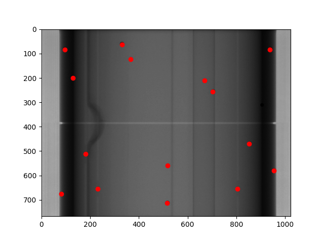
For example, here is an example analysis of an MPC image:

from pylinac.core.image import XIM
from pylinac.core.metrics import GlobalDiskLocator

img = XIM("my_image.xim")
bbs = img.compute(
    metrics=GlobalDiskLocator(
        radius_mm=3.5,
        radius_tolerance_mm=1.5,
        min_number=10,
    )
)
img.plot()

This will result in an image like so:

Global Sized Field Locator#

New in version 3.17.

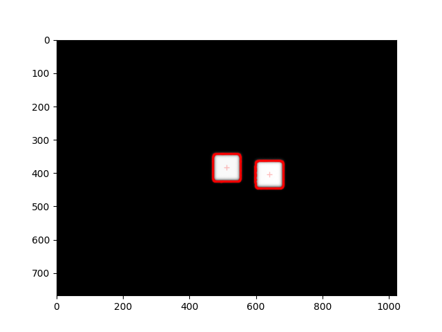
The GlobalSizedFieldLocator metric is similar to the GlobalDiskLocator metric except that it searches the entire image for fields of a given size. This is useful for finding one or more fields in images where the field is not in the expected location or unknown. This is also efficient when multiple fields are present in the image.

The locator will find the weighted center of the field(s) and return the location(s) as a Point objects. The boundary of the detected field(s) will be plotted on the image in addition to the center.

The locator will use pixels by default, but also has a from_physical class method to use physical units.

An example plot of finding multiple fields can be seen below:

../_images/global_sized_field_locator.png

For example:

Search for at least 2 fields of size 30x30 pixels with a tolerance of 4 pixels & plot#

img = DicomImage("my_image.dcm")
img.compute(
    metrics=GlobalSizedFieldLocator(
        field_width_px=30, field_height_px=30, field_tolerance_px=4, max_number=2
    )
)
img.plot()  # this will plot the image with the fields overlaid

Using physical units#

To perform a similar field location using mm instead of pixels:

Search for at least 2 fields of size 30x30mm with a tolerance of 4mm#

img = DicomImage("my_image.dcm")
img.compute(
    metrics=GlobalSizedFieldLocator.from_physical(
        field_width_mm=30, field_height_mm=30, field_tolerance_mm=4, max_number=2
    )
)

Usage tips#

Whenever possible, set the max_number parameter. This can greatly speed up the computation for several reasons. First, it will stop searching once the number of fields is found. Second, the thresholding algorithm will have a much better initial guess and also a better step size. This is because the approximate area of the field is known relative to the total image size.
The field_tolerance_<mm|px> parameter can be relatively tight if the max_number parameter is set. Without a max_number parameter, you may have to increase the field tolerance to find all fields.

Writing Custom Plugins#

The power of the plugin architecture is that you can write your own metrics and use them on any image as well as reuse them where needed.

To write a custom plugin, you must

Inherit from the MetricBase class
Specify a name attribute.
Implement the calculate method.
(Optional) Implement the plot method if you want the metric to plot on the image.

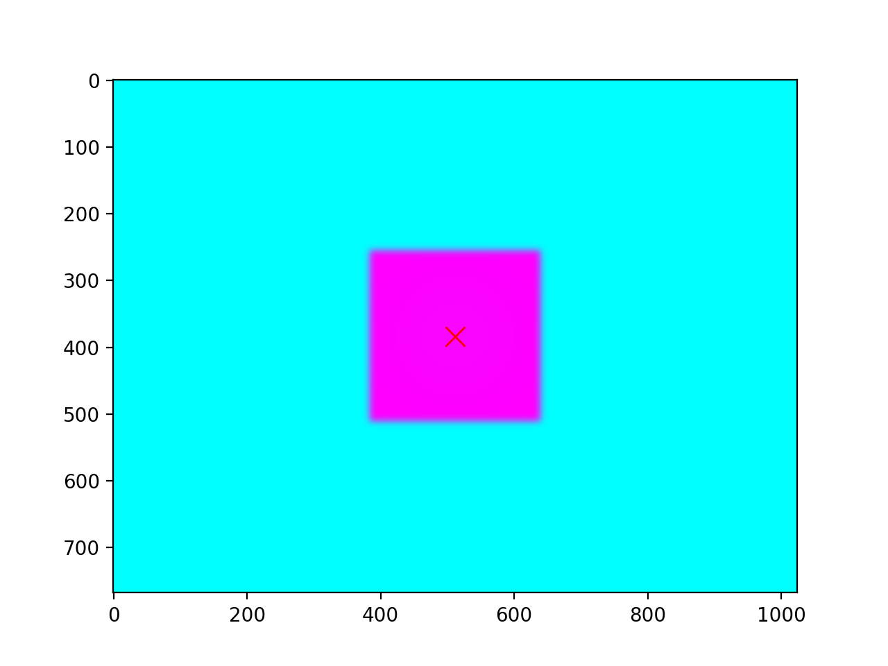
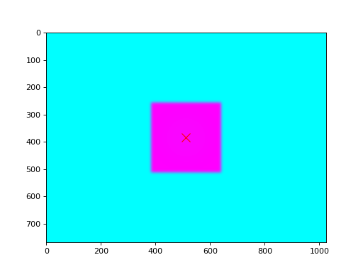
For example, let’s built a simple plugin that finds and plots an “X” at the center of the image:

from pylinac.core.image_generator import AS1000Image, FilteredFieldLayer, GaussianFilterLayer
from pylinac.core.image import DicomImage
from pylinac.core.metrics import MetricBase

class ImageCenterMetric(MetricBase):
    name = "Image Center"

    def calculate(self):
        return self.image.center

    def plot(self, axis: plt.Axes):
        axis.plot(self.image.center.x, self.image.center.y, 'rx', markersize=10)

# now we create an image to compute over
as1000 = AS1000Image(sid=1000)  # this will set the pixel size and shape automatically
as1000.add_layer(
    FilteredFieldLayer(field_size_mm=(100, 100))
)  # create a 100x100mm square field
as1000.add_layer(
    GaussianFilterLayer(sigma_mm=2)
)  # add an image-wide gaussian to simulate penumbra/scatter
ds = as1000.as_dicom()

# now we can compute the metric on the image
img = DicomImage.from_dataset(ds)
center = img.compute(metrics=ImageCenterMetric())
print(center)
img.plot()

(Source code, png, hires.png, pdf)

API#

class pylinac.core.metrics.MetricBase[source]#

Bases: ABC

Base class for any 2D metric. This class is abstract and should not be instantiated.

The subclass should implement the calculate method and the name attribute.

As a best practice, the image_compatibility attribute should be set to a list of image classes that the metric is compatible with. Image types that are not in the list will raise an error. This allows compatibility to be explicit. However, by default this is None and no compatibility checking is done.

inject_image(image: BaseImage)[source]#: Inject the image into the metric.

context_calculate() → Any[source]#

Calculate the metric, passing in an image copy so that modifications to the image don’t affect the original.

This is also kinda memory efficient since the original image is a reference. The copy here will get destroyed after the call returns vs keeping a copy around.

So at any given time, only 2x the memory is required instead of Nx. This is important when computing multiple metrics.

abstract calculate() → Any[source]#: Calculate the metric. Can return anything

plot(axis: Axes) → None[source]#: Plot the metric

additional_plots() → list[figure][source]#

Plot additional information on a separate figure as needed.

This should NOT show the figure. The figure will be shown via the metric_plots method. Calling show here would block other metrics from plotting their own separate metrics.

class pylinac.core.metrics.DiskLocator(expected_position: Point | tuple[float, float], search_window: tuple[float, float], radius: float, radius_tolerance: float, detection_conditions: list[Callable[[RegionProperties, ...], bool]] = (<function is_round>, <function is_right_size_bb>, <function is_right_circumference>), name: str = 'Disk Region')[source]#

Bases: DiskRegion

Calculates the weighted centroid of a disk/BB as a Point in an image where the disk is near an expected position and size.

calculate() → Point[source]#: Get the weighted centroid of the region prop of the BB.

plot(axis: Axes) → None[source]#: Plot the BB center

additional_plots() → list[figure]#

Plot additional information on a separate figure as needed.

This should NOT show the figure. The figure will be shown via the metric_plots method. Calling show here would block other metrics from plotting their own separate metrics.

context_calculate() → Any#

Calculate the metric, passing in an image copy so that modifications to the image don’t affect the original.

This is also kinda memory efficient since the original image is a reference. The copy here will get destroyed after the call returns vs keeping a copy around.

So at any given time, only 2x the memory is required instead of Nx. This is important when computing multiple metrics.

classmethod from_center(expected_position: Point | tuple[float, float], search_window: tuple[float, float], radius: float, radius_tolerance: float, detection_conditions: list[Callable[[RegionProperties, ...], bool]] = (<function is_round>, <function is_right_size_bb>, <function is_right_circumference>), name='Disk Region')#: Create a DiskRegion from a center point.

classmethod from_center_physical(expected_position_mm: Point | tuple[float, float], search_window_mm: tuple[float, float], radius_mm: float, radius_tolerance_mm: float = 0.25, detection_conditions: list[Callable[[RegionProperties, ...], bool]] = (<function is_round>, <function is_right_size_bb>, <function is_right_circumference>), name='Disk Region')#: Create a DiskRegion using physical dimensions from the center point.

classmethod from_physical(expected_position_mm: Point | tuple[float, float], search_window_mm: tuple[float, float], radius_mm: float, radius_tolerance_mm: float, detection_conditions: list[Callable[[RegionProperties, ...], bool]] = (<function is_round>, <function is_right_size_bb>, <function is_right_circumference>), name='Disk Region')#: Create a DiskRegion using physical dimensions.

inject_image(image: BaseImage)#: Inject the image into the metric.

class pylinac.core.metrics.DiskRegion(expected_position: Point | tuple[float, float], search_window: tuple[float, float], radius: float, radius_tolerance: float, detection_conditions: list[Callable[[RegionProperties, ...], bool]] = (<function is_round>, <function is_right_size_bb>, <function is_right_circumference>), name: str = 'Disk Region')[source]#

Bases: MetricBase

A metric to find a disk/BB in an image where the BB is near an expected position and size. This will calculate the scikit-image regionprops of the BB.

classmethod from_physical(expected_position_mm: Point | tuple[float, float], search_window_mm: tuple[float, float], radius_mm: float, radius_tolerance_mm: float, detection_conditions: list[Callable[[RegionProperties, ...], bool]] = (<function is_round>, <function is_right_size_bb>, <function is_right_circumference>), name='Disk Region')[source]#: Create a DiskRegion using physical dimensions.

classmethod from_center(expected_position: Point | tuple[float, float], search_window: tuple[float, float], radius: float, radius_tolerance: float, detection_conditions: list[Callable[[RegionProperties, ...], bool]] = (<function is_round>, <function is_right_size_bb>, <function is_right_circumference>), name='Disk Region')[source]#: Create a DiskRegion from a center point.

classmethod from_center_physical(expected_position_mm: Point | tuple[float, float], search_window_mm: tuple[float, float], radius_mm: float, radius_tolerance_mm: float = 0.25, detection_conditions: list[Callable[[RegionProperties, ...], bool]] = (<function is_round>, <function is_right_size_bb>, <function is_right_circumference>), name='Disk Region')[source]#: Create a DiskRegion using physical dimensions from the center point.

calculate() → RegionProperties[source]#

Find the scikit-image regiongprops of the BB.

This will apply a high-pass filter to the image iteratively. The filter starts at a very low percentile and increases until a region is found that meets the detection conditions.

additional_plots() → list[figure]#

Plot additional information on a separate figure as needed.

This should NOT show the figure. The figure will be shown via the metric_plots method. Calling show here would block other metrics from plotting their own separate metrics.

context_calculate() → Any#

Calculate the metric, passing in an image copy so that modifications to the image don’t affect the original.

This is also kinda memory efficient since the original image is a reference. The copy here will get destroyed after the call returns vs keeping a copy around.

So at any given time, only 2x the memory is required instead of Nx. This is important when computing multiple metrics.

inject_image(image: BaseImage)#: Inject the image into the metric.

plot(axis: Axes) → None#: Plot the metric

class pylinac.core.metrics.GlobalDiskLocator(radius_mm: float, radius_tolerance_mm: float, detection_conditions: list[Callable[[RegionProperties, ...], bool]] = (<function is_round>, <function is_right_size_bb>, <function is_right_circumference>), min_number: int = 1, max_number: int | None = None, min_separation_mm: float = 5, name='Global Disk Locator')[source]#

Bases: MetricBase

Finds BBs globally within an image.

Parameters#

radius_mmfloat: The radius of the BB in mm.
radius_tolerance_mmfloat: The tolerance of the BB radius in mm.
detection_conditionslist[callable]: A list of functions that take a regionprops object and return a boolean. The functions should be used to determine whether the regionprops object is a BB.
min_numberint: The minimum number of BBs to find. If not found, an error is raised.
max_numberint, None: The maximum number of BBs to find. If None, no maximum is set.
min_separation_mmfloat: The minimum distance between BBs in mm. If BBs are found that are closer than this, they are deduplicated.
namestr: The name of the metric.

calculate() → list[Point][source]#: Find up to N BBs/disks in the image. This will look for BBs at every percentile range. Multiple BBs may be found at different threshold levels.

plot(axis: Axes) → None[source]#: Plot the BB centers

additional_plots() → list[figure]#

Plot additional information on a separate figure as needed.

This should NOT show the figure. The figure will be shown via the metric_plots method. Calling show here would block other metrics from plotting their own separate metrics.

context_calculate() → Any#

Calculate the metric, passing in an image copy so that modifications to the image don’t affect the original.

This is also kinda memory efficient since the original image is a reference. The copy here will get destroyed after the call returns vs keeping a copy around.

So at any given time, only 2x the memory is required instead of Nx. This is important when computing multiple metrics.

inject_image(image: BaseImage)#: Inject the image into the metric.

class pylinac.core.metrics.GlobalSizedFieldLocator(field_width_px: float, field_height_px: float, field_tolerance_px: float, min_number: int = 1, max_number: int | None = None, name: str = 'Field Finder', detection_conditions: list[callable] = (<function is_right_square_perimeter>, <function is_right_area_square>), default_threshold_step_size: float = 2)[source]#

Bases: MetricBase

Finds fields globally within an image.

Parameters#

field_width_pxfloat: The width of the field in px.
field_height_pxfloat: The height of the field in px.
field_tolerance_pxfloat: The tolerance of the field size in px.
min_numberint: The minimum number of fields to find. If not found, an error is raised.
max_numberint, None: The maximum number of fields to find. If None, no maximum is set.
namestr: The name of the metric.
detection_conditionslist[callable]: A list of functions that take a regionprops object and return a boolean.
default_threshold_step_sizefloat: The default step size for the threshold iteration. This is based on the max number of fields and the field size.

classmethod from_physical(field_width_mm: float, field_height_mm: float, field_tolerance_mm: float, min_number: int = 1, max_number: int | None = None, name: str = 'Field Finder', detection_conditions: list[callable] = (<function is_right_square_perimeter>, <function is_right_area_square>), default_threshold_step_size: float = 2)[source]#

Construct an instance using physical dimensions.

Parameters#

field_width_mmfloat: The width of the field in mm.
field_height_mmfloat: The height of the field in mm.
field_tolerance_mmfloat: The tolerance of the field size in mm.
min_numberint: The minimum number of fields to find. If not found, an error is raised.
max_numberint, None: The maximum number of fields to find. If None, no maximum is set.
namestr: The name of the metric.
detection_conditionslist[callable]: A list of functions that take a regionprops object and return a boolean.
default_threshold_step_sizefloat: The default step size for the threshold iteration. This is based on the max number of fields and the field size.

property threshold_step_size: float#: Set the step size for the threshold. This is based on the max number of fields and the field size.

additional_plots() → list[figure]#

Plot additional information on a separate figure as needed.

This should NOT show the figure. The figure will be shown via the metric_plots method. Calling show here would block other metrics from plotting their own separate metrics.

context_calculate() → Any#

Calculate the metric, passing in an image copy so that modifications to the image don’t affect the original.

This is also kinda memory efficient since the original image is a reference. The copy here will get destroyed after the call returns vs keeping a copy around.

So at any given time, only 2x the memory is required instead of Nx. This is important when computing multiple metrics.

inject_image(image: BaseImage)#: Inject the image into the metric.

property threshold_start: float#: The starting percentile for the threshold. This is based on the max number of fields and the field size.

calculate() → list[Point][source]#: Find up to N fields in the image. This will look for fields at every percentile range. Multiple fields may be found at different threshold levels.

plot(axis: Axes, show_boundaries: bool = True, color: str = 'red', markersize: float = 3, alpha: float = 0.25) → None[source]#: Plot the BB centers and boundary of detection.