Winston-Lutz Multi-Target#

Overview#

New in version 3.9.

The Multi-Target Winston-Lutz (MTWL) is an advanced test category meant to measure multiple locations away from isocenter, typically to represent multi-lesion SRS cases. The MTWL module can analyze images with any number of BBs in any arrangement. It is generalizable such that new phantom analyses can be created quickly.

Technically, there are two flavors of multi-target WL: multi-field and single field. An example of a multi-field WL is the SNC MultiMet. Each field is centered around each BB. The BB position is compared to that of the field. This is closest to what the patient experiences since it incorporates both the gantry/coll/couch deviations as well as the MLCs.

An example of a single-field multi-target WL is Machine Performance Check. The BBs are compared to the known positions. This removes the error of the MLCs to isolate just the gantry/coll/couch.

Currently, only the multi-field flavor is supported, but work on the single-field flavor will occur to support things like secondary checks of MPC.

This is why the class is called WinstonLutzMultiTargetMultiField as there will be an anticipated WinstonLutzMultiTargetSingleField.

Differences from single-target WL#

Warning

The MTWL algorithm is new and provisional. There are a number of limitations with the algorithm. Hopefully, these are removed in future updates. The algorithm is still considered valuable even with these limitations which is why it is released.

Important

In a nutshell, the MTWL analyzes BB positions only, whereas vanilla WL provides more machine-related data as well as BB position data.

Unlike the single-target WL algorithm (aka “vanilla” WL), there are more limitations to acquisition and outputs. This should improve over time, but for now you can think of the MTWL as a subset of the vanilla WL algorithm:

Utility methods such as loading images are the same.
Outputs related to the BBs are different.
BB size is not a parameter but is part of the BB arrangement.
Single images cannot be analyzed.
Axis deviations (Gantry wobble, etc) are not yet available.
Couch rotation images are dropped as they cannot yet be handled.
Interpreting filenames is not yet allowed.

See the following sections for more info.

Image Acquisition
Supported Phantoms

Running the Demo#

To run the multi-target Winston-Lutz demo, create a script or start an interpreter session and input:

from pylinac import WinstonLutzMultiTargetMultiField

WinstonLutzMultiTargetMultiField.run_demo()

Results will be printed to the console and a figure showing the zoomed-in images will be generated:

Winston-Lutz Multi-Target Multi-Field Analysis
==============================================
Number of images: 4

2D distances
============
Max 2D distance of any BB: 0.00 mm
Mean 2D distance of any BB: 0.00 mm
Median 2D distance of any BB: 0.00 mm

  BB #  Description
------  ---------------------------------------------
     0  'Iso': Left 0mm, Up 0mm, In 0mm
     1  'Left,Down,In': Left 20mm, Down 20mm, In 60mm

Image                   G    Co    Ch    BB #0    BB #1
--------------------  ---  ----  ----  -------  -------
=0, Gantry sag=0.dcm    0     0     0        0        0
=0, Gantry sag=0.dcm   90     0     0        0        0
=0, Gantry sag=0.dcm  180     0     0        0        0
=0, Gantry sag=0.dcm  270     0     0        0        0

(Source code)

_images/winston_lutz_multi-1_00.png — (`png`, `hires.png`, `pdf`)#

_images/winston_lutz_multi-1_01.png — (`png`, `hires.png`, `pdf`)#

Image Acquisition#

The Winston-Lutz module will only load EPID images. The images can be from any EPID however and any SID. To ensure the most accurate results the following should be noted:

Images with a rotated couch are dropped and not analyzed (yet) but will not cause an error.
The BBs should not occlude each other.
The BBs should be >5mm apart in any given image.
The radiation fields should have >5mm separation in any given image.
The BB and radiation field should be <=5 mm away from the nominal location given by the arrangement.

Coordinate Space#

The MTWL algorithm uses the same coordinate system as the vanilla WL. Coordinate Space.

Passing a coordinate system#

No coordinate system is passed or used (yet).

Note

This is a target for the MTWL algorithm, so expect this to change in the future.

Supported Phantoms#

Currently, only the MultiMet-WL cube from SNC is supported. However, the algorithm is generalized and can be easily adapted to analyze other phantoms. See Custom BB Arrangements.

Typical Use#

Analyzing a multi-target Winston-Lutz test is simple. First, let’s import the class:

from pylinac import WinstonLutzMultiTargetMultiField
from pylinac.winston_lutz import BBArrangement

From here, you can load a directory:

my_directory = "path/to/wl_images"
wl = WinstonLutzMultiTargetMultiField(my_directory)

You can also load a ZIP archive with the images in it:

wl = WinstonLutzMultiTargetMultiField.from_zip("path/to/wl.zip")

Now, analyze it. Unlike the vanilla WL algorithm, we have to pass the BB arrangement to know where the BBs should be in space. Preset phantoms exist, or a custom arrangement can be passed.

wl.analyze(bb_arrangement=BBArrangement.SNC_MULTIMET)

And that’s it! You can now view images, print the results, or publish a PDF report:

# plot all the images
wl.plot_images()
# save figures of the image plots for each bb
wl.save_images(prefix="snc")
# print to PDF
wl.publish_pdf("mymtwl.pdf")

Changing BB detection size#

To change the size of BB pylinac is expecting you must change it in the BB arrangement. This allows phantoms with multiple BB sizes to still be analyzed. See Custom BB Arrangements

Custom BB Arrangements#

The MTWL algorithm uses a priori BB arrangements. I.e. you need to know where the BBs should exist in space relative to isocenter. The MTWL algorithm is flexible to accommodate any reasonable arrangement of BBs.

To create a custom arrangement, say for an in-house phantom or commercial phantom not yet supported, define the BB offsets and size like so. Use negative values to move the other direction:

my_special_phantom_bbs = [
    {
        "offset_left_mm": 0,
        "offset_up_mm": 0,
        "offset_in_mm": 0,
        "bb_size_mm": 5,
        "rad_size_mm": 20,
    },  # 5mm BB at iso
    {
        "offset_left_mm": 30,
        "offset_up_mm": 0,
        "offset_in_mm": 0,
        "bb_size_mm": 4,
        "rad_size_mm": 20,
    },  # 4mm BB 30mm to left of iso
    {
        "offset_left_mm": 0,
        "offset_up_mm": -20,
        "offset_in_mm": 10,
        "bb_size_mm": 5,
        "rad_size_mm": 20,
    },  # BB DOWN 20mm and in 10mm
    ...,  # keep going as needed
]

Pass it to the algorithm like so:

wl = WinstonLutzMultiTargetMultiField(...)
wl.analyze(bb_arrangement=my_special_phantom_bbs)
...

Algorithm#

The MTWL algorithm is based on the vanilla WL algorithm. For each BB and image combination, the image is searched at the nominal location for the BB and radiation field. If it’s not found it will be skipped for that combo. The BB must be detected in at least one image or an error will be raised.

The algorithm works like such:

Allowances

The images can be acquired with any EPID (aS500, aS1000, aS1200) at any SID.
The image can have any number of BBs.
The BBs can be at any 3D location.

Restrictions

Warning

Analysis can fail or give unreliable results if any Restriction is violated.

Each BB and radiation field must be within 5mm of the expected position in x and y in the EPID plane. I.e. it must be <=7mm in scalar distance.
BBs must not occlude or be <5 mm from each other in any 2D image.
Images with a rotated couch are dropped and not analyzed (yet) but will not cause an error.
The radiation fields should have >5mm separation in any given image.

Analysis

This algorithm is performed for each BB and image combination:

Find the field center – The spread in pixel values (max - min) is divided by 2, and any pixels above the threshold is associated with the open field. The pixels are converted to black & white and the center of mass of the pixels is assumed to be the field center.
Find the BB – The image is converted to binary based on pixel values both above the 50% threshold as above, and below the upper threshold. The upper threshold is an iterative value, starting at the image maximum value, that is lowered slightly when the BB is not found. If the binary image has a reasonably circular ROI, is approximately the right size, and is within 5mm of the expected BB position, the BB is considered found and the pixel-weighted center of mass of the BB is considered the BB location.
Evaluate against the field position – Once the measured BB and field positions are known, both the scalar distance and vector from the field position to the measured BB position is determined.

Benchmarking the Algorithm#

With the image generator module we can create test images to test the WL algorithm on known results. This is useful to isolate what is or isn’t working if the algorithm doesn’t work on a given image and when commissioning pylinac. It is common, especially with the WL module, to question the accuracy of the algorithm. Since no linac is perfect and the results are sub-millimeter, discerning what is true error vs algorithmic error can be difficult. The image generator module is a perfect solution since it can remove or reproduce the former error.

Note

With the introduction of the MTWL algorithm, so to a multi-target synthetic image generator has been created: generate_winstonlutz_multi_bb_multi_field().

Warning

The image generator is limited in accuracy to ~1/2 pixel because creating the image requires a row or column to be set. E.g. a 5mm field with a 0.336mm pixel size means we need to create a field of 14.88 pixels wide. We can only set the field to be 14 or 15 pixels, so the nearest field size of 15 pixels or 5.04mm is set.

2-BB Perfect Delivery#

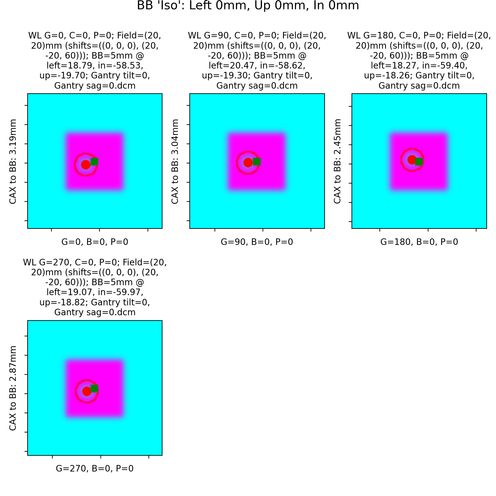
Create a perfect set of fields with 1 BB at iso and another 20mm left, 20mm down, and 60mm inward (this is the same as the demo, but is good for explanation).

import pylinac
from pylinac.core.image_generator import simulators, layers, generate_winstonlutz_multi_bb_multi_field

wl_dir = 'wl_dir'
generate_winstonlutz_multi_bb_multi_field(
        simulator=simulators.AS1200Image(sid=1000),
        field_layer=layers.PerfectFieldLayer,
        final_layers=[layers.GaussianFilterLayer(sigma_mm=1),],
        dir_out=wl_dir,
        field_offsets=((0, 0, 0), (20, -20, 60)),
        field_size_mm=(20, 20),
        bb_offsets=[[0, 0, 0], [20, -20, 60]],
)
arrange = (
    {'name': 'Iso', 'offset_left_mm': 0, 'offset_up_mm': 0, 'offset_in_mm': 0, 'bb_size_mm': 5, 'rad_size_mm': 20},
    {'name': 'Left,Down,In', 'offset_left_mm': 20, 'offset_up_mm': -20, 'offset_in_mm': 60, 'bb_size_mm': 5, 'rad_size_mm': 20},)

wl = pylinac.WinstonLutzMultiTargetMultiField(wl_dir)
wl.analyze(bb_arrangement=arrange)
print(wl.results())
wl.plot_images()

(Source code)

_images/winston_lutz_multi-2_00.png — (`png`, `hires.png`, `pdf`)#

_images/winston_lutz_multi-2_01.png — (`png`, `hires.png`, `pdf`)#

which has an output of:

Winston-Lutz Multi-Target Multi-Field Analysis
==============================================
Number of images: 4

2D distances
============
Max 2D distance of any BB: 0.00 mm
Mean 2D distance of any BB: 0.00 mm
Median 2D distance of any BB: 0.00 mm

  BB #  Description
------  ---------------------------------------------
     0  'Iso': Left 0mm, Up 0mm, In 0mm
     1  'Left,Down,In': Left 20mm, Down 20mm, In 60mm

Image                   G    Co    Ch    BB #0    BB #1
--------------------  ---  ----  ----  -------  -------
=0, Gantry sag=0.dcm    0     0     0        0        0
=0, Gantry sag=0.dcm   90     0     0        0        0
=0, Gantry sag=0.dcm  180     0     0        0        0
=0, Gantry sag=0.dcm  270     0     0        0        0

As shown, we have perfect results.

Offset BBs#

Let’s now offset both BBs by 1mm to the left:

import pylinac
from pylinac.core.image_generator import simulators, layers, generate_winstonlutz_multi_bb_multi_field

wl_dir = 'wl_dir'
generate_winstonlutz_multi_bb_multi_field(
        simulator=simulators.AS1200Image(sid=1000),
        field_layer=layers.PerfectFieldLayer,
        final_layers=[layers.GaussianFilterLayer(sigma_mm=1),],
        dir_out=wl_dir,
        field_offsets=((0, 0, 0), (20, -20, 60)),
        field_size_mm=(20, 20),
        bb_offsets=[[1, 0, 0], [19, -20, 60]],  # here's the offset
)
arrange = (
    {'name': 'Iso', 'offset_left_mm': 0, 'offset_up_mm': 0, 'offset_in_mm': 0, 'bb_size_mm': 5, 'rad_size_mm': 20},
    {'name': 'Left,Down,In', 'offset_left_mm': 20, 'offset_up_mm': -20, 'offset_in_mm': 60, 'bb_size_mm': 5, 'rad_size_mm': 20},)

wl = pylinac.WinstonLutzMultiTargetMultiField(wl_dir)
wl.analyze(bb_arrangement=arrange)
print(wl.results())
wl.plot_images()

(Source code)

_images/winston_lutz_multi-3_00.png — (`png`, `hires.png`, `pdf`)#

_images/winston_lutz_multi-3_01.png — (`png`, `hires.png`, `pdf`)#

with an output of:

Winston-Lutz Multi-Target Multi-Field Analysis
==============================================
Number of images: 4

2D distances
============
Max 2D distance of any BB: 1.01 mm
Mean 2D distance of any BB: 1.01 mm
Median 2D distance of any BB: 1.01 mm

  BB #  Description
------  ---------------------------------------------
     0  'Iso': Left 0mm, Up 0mm, In 0mm
     1  'Left,Down,In': Left 20mm, Down 20mm, In 60mm

Image                   G    Co    Ch    BB #0    BB #1
--------------------  ---  ----  ----  -------  -------
=0, Gantry sag=0.dcm    0     0     0     1.01     1.01
=0, Gantry sag=0.dcm   90     0     0     0        0
=0, Gantry sag=0.dcm  180     0     0     1.01     1.01
=0, Gantry sag=0.dcm  270     0     0     0        0

Both BBs report a shift of 1mm. Note this is only in 0 and 180. A left shift would not be captured at 90/270.

Random error#

Let’s now add random error:

Note

The error is random so performing this again will change the results slightly.

import pylinac
from pylinac.core.image_generator import simulators, layers, generate_winstonlutz_multi_bb_multi_field

wl_dir = 'wl_dir'
generate_winstonlutz_multi_bb_multi_field(
        simulator=simulators.AS1200Image(sid=1000),
        field_layer=layers.PerfectFieldLayer,
        final_layers=[layers.GaussianFilterLayer(sigma_mm=1),],
        dir_out=wl_dir,
        field_offsets=((0, 0, 0), (20, -20, 60)),
        field_size_mm=(20, 20),
        bb_offsets=[[0, 0, 0], [20, -20, 60]],
        jitter_mm=2  # here we add random noise
)
arrange = (
    {'name': 'Iso', 'offset_left_mm': 0, 'offset_up_mm': 0, 'offset_in_mm': 0, 'bb_size_mm': 5, 'rad_size_mm': 20},
    {'name': 'Left,Down,In', 'offset_left_mm': 20, 'offset_up_mm': -20, 'offset_in_mm': 60, 'bb_size_mm': 5, 'rad_size_mm': 20},)

wl = pylinac.WinstonLutzMultiTargetMultiField(wl_dir)
wl.analyze(bb_arrangement=arrange)
print(wl.results())
wl.plot_images()

(Source code)

_images/winston_lutz_multi-4_00.png — (`png`, `hires.png`, `pdf`)#

_images/winston_lutz_multi-4_01.png — (`png`, `hires.png`, `pdf`)#

with an output of:

Winston-Lutz Multi-Target Multi-Field Analysis
==============================================
Number of images: 4

2D distances
============
Max 2D distance of any BB: 3.38 mm
Mean 2D distance of any BB: 2.82 mm
Median 2D distance of any BB: 2.82 mm

  BB #  Description
------  ---------------------------------------------
     0  'Iso': Left 0mm, Up 0mm, In 0mm
     1  'Left,Down,In': Left 20mm, Down 20mm, In 60mm

Image                   G    Co    Ch    BB #0    BB #1
--------------------  ---  ----  ----  -------  -------
=0, Gantry sag=0.dcm    0     0     0     2.25     0.34
=0, Gantry sag=0.dcm   90     0     0     2.15     2.77
=0, Gantry sag=0.dcm  180     0     0     2.13     3.38
=0, Gantry sag=0.dcm  270     0     0     2.25     2.42

API Documentation#

class pylinac.winston_lutz.WinstonLutzMultiTargetMultiField(*args, **kwargs)[source]#

Bases: WinstonLutz

We cannot yet handle non-0 couch angles so we drop them. Analysis fails otherwise

analyzed_images: dict[str, list[WinstonLutz2DMultiTarget]]#

image_type#: alias of WinstonLutz2DMultiTarget

bb_arrangement: Sequence[dict]#

images: Sequence[WinstonLutz2DMultiTarget]#

classmethod from_demo_images()[source]#: Instantiate using the demo images.

static run_demo()[source]#: Run the Winston-Lutz MT MF demo, which loads the demo files, prints results, and plots a summary image.

analyze(bb_arrangement: Sequence[dict])[source]#

Analyze the WL images.

Parameters#

bb_arrangement: The arrangement of the BBs in the phantom. A dict with offset and BB size keys. See the BBArrangement class for keys and syntax.

plot_images(show: bool = True, **kwargs)[source]#: Make a plot for each BB. Each plot contains the analysis of that BB on each image it was found.

save_images(prefix: str = '', **kwargs)[source]#

Save the figure of plot_images() to file as PNG. Keyword arguments are passed to matplotlib.pyplot.savefig().

Parameters#

prefixstr: The prefix name of the file to save to. The BB name is appended to the prefix.

save_images_to_stream(**kwargs) → dict[str, BytesIO][source]#: Save the individual image plots to stream

cax2bb_distance(bb: str, metric: str = 'max') → float[source]#

The distance in mm between the CAX and BB for all images according to the given metric.

Parameters#

metric{‘max’, ‘median’, ‘mean’}: The metric of distance to use.
bbstr: The BB to analyze

results_data(as_dict: bool = False) → WinstonLutzMultiTargetMultiFieldResult | dict[source]#: Present the results data and metadata as a dataclass or dict. The default return type is a dataclass.

plot_summary(show: bool = True, fig_size: tuple | None = None)[source]#: Plot a summary figure showing the gantry sag and wobble plots of the three axes.

plot_axis_images(axis: Axis = Axis.GANTRY, show: bool = True, ax: plt.Axes | None = None)[source]#

Plot all CAX/BB/EPID positions for the images of a given axis.

For example, axis=’Couch’ plots a reference image, and all the BB points of the other images where the couch was moving.

Parameters#

axis{‘Gantry’, ‘Collimator’, ‘Couch’, ‘GB Combo’, ‘GBP Combo’}: The images/markers from which accelerator axis to plot.
showbool: Whether to actually show the images.
axNone, matplotlib.Axes: The axis to plot to. If None, creates a new plot.

property max_bb_deviation_2d: float#: The maximum distance from any measured BB to its nominal position

property mean_bb_deviation_2d: float#: The mean distance from any measured BB to its nominal position

property median_bb_deviation_2d: float#: The median distance from any measured BB to its nominal position

results(as_list: bool = False) → str[source]#

Return the analysis results summary.

Parameters#

as_listbool: Whether to return as a list of strings vs single string. Pretty much for internal usage.

Publish (print) a PDF containing the analysis, images, and quantitative results.

Parameters#

filename(str, file-like object): The file to write the results to.
notesstr, list of strings: Text; if str, prints single line. If list of strings, each list item is printed on its own line.
open_filebool: Whether to open the file using the default program after creation.
metadatadict: Extra data to be passed and shown in the PDF. The key and value will be shown with a colon. E.g. passing {‘Author’: ‘James’, ‘Unit’: ‘TrueBeam’} would result in text in the PDF like: ————– Author: James Unit: TrueBeam ————–
logo: Path, str: A custom logo to use in the PDF report. If nothing is passed, the default pylinac logo is used.

class pylinac.winston_lutz.WinstonLutz2DMultiTarget(*args, **kwargs)[source]#

Bases: WinstonLutz2D

A 2D image of a WL delivery, but where multiple BBs are in use.

Parameters#

filestr: Path to the image file.
use_filenames: bool: Whether to try to use the file name to determine axis values. Useful for Elekta machines that do not include that info in the DICOM data.

as_analyzed(bb_location: dict) → WinstonLutz2DMultiTarget[source]#

Analyze the image of the multi-BB setup. We return a copy of the WL image because we analyze images more than once. Each “analyzed” image is really the analysis of a BB/image combo.

Parameters#

bb_location: An iterable of dictionaries. Each dict contains keys for the offsets and size of the BB in mm. Use the BBArrangement class as a guide.

plot(ax: plt.Axes | None = None, show: bool = True, clear_fig: bool = False) → plt.Axes[source]#

Plot the image, zoomed-in on the radiation field, along with the detected BB location and field CAX location.

Parameters#

axNone, matplotlib Axes instance: The axis to plot to. If None, will create a new figure.
showbool: Whether to actually show the image.
clear_figbool: Whether to clear the figure first before drawing.

location_near_nominal(region: RegionProperties, location: dict) → bool[source]#: Determine whether the given BB ROI is near where the BB is expected to be

results_data(as_dict: bool = False) → WinstonLutz2DResult | dict[source]#: Present the results data and metadata as a dataclass or dict. The default return type is a dataclass.

class pylinac.winston_lutz.WinstonLutzMultiTargetMultiFieldResult(num_total_images: int, max_2d_field_to_bb_mm: float, median_2d_field_to_bb_mm: float, mean_2d_field_to_bb_mm: float, bb_arrangement: Iterable[dict], bb_maxes: dict)[source]#

Bases: ResultBase

This class should not be called directly. It is returned by the results_data() method. It is a dataclass under the hood and thus comes with all the dunder magic.

Use the following attributes as normal class attributes.

num_total_images: int#

max_2d_field_to_bb_mm: float#

median_2d_field_to_bb_mm: float#

mean_2d_field_to_bb_mm: float#

bb_arrangement: Iterable[dict]#

bb_maxes: dict#